API Tutorial For Beginners With Google Sheets & Apps Script

In this API tutorial for beginners, you’ll learn how to connect to APIs using Google Apps Script, to retrieve data from a third-party and display it in your Google Sheet.

Example 1 shows you how to use Google Apps Script to connect to a simple API to retrieve some data and show it in Google Sheets:

API tutorial for beginners: Random math facts from Numbers API in Google Sheet

In Example 2, we’ll use Google Apps Script to build a music discovery application using the iTunes API:

Itunes API with Google Sheets

Finally, in example 3, I’ll leave you to have a go at building a Star Wars data explorer application, with a few hints:

Star Wars API explorer in Google Sheets using Google Apps Script

API tutorial for beginners: what is an API?

You’ve probably heard the term API before. Maybe you’ve heard how tech companies use them when they pipe data between their applications. Or how companies build complex systems from many smaller micro-services linked by APIs, rather than as single, monolithic programs nowadays.

API stands for “Application Program Interface”, and the term commonly refers to web URLs that can be used to access raw data. Basically, the API is an interface that provides raw data for the public to use (although many require some form of API authentication).

As third-party software developers, we can access an organization’s API and use their data within our own applications.

The good news is that there are plenty of simple APIs out there, which we can cut our teeth on. We’ll see three of them in this beginner api tutorial.

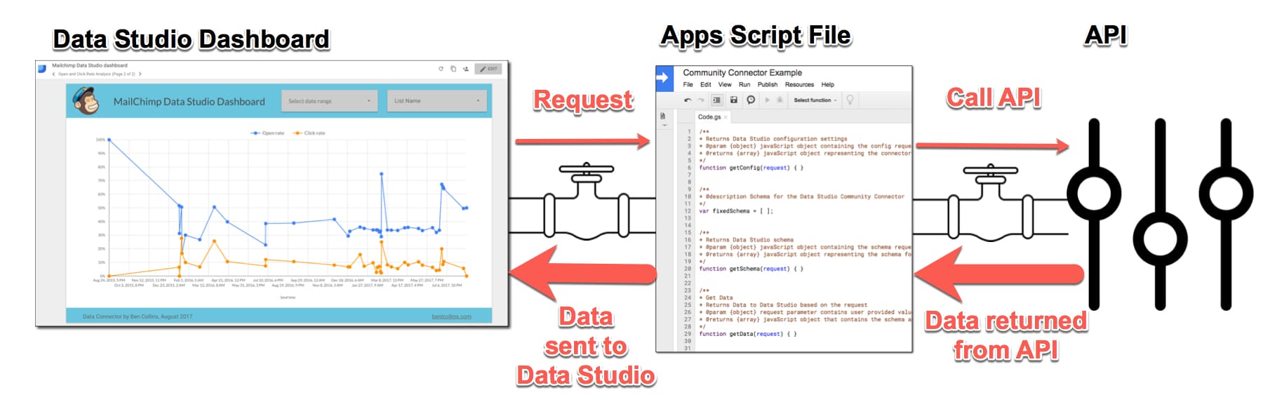
We can connect a Google Sheet to an API and bring data back from that API (e.g. iTunes) into our Google Sheet using Google Apps Script. It’s fun and really satisfying if you’re new to this world.

API tutorial for beginners: what is Apps Script?

In this API tutorial for beginners, we’ll use Google Apps Script to connect to external APIs.

Google Apps Script is a Javascript-based scripting language hosted and run on Google servers, that extends the functionality of Google Apps.

If you’ve never used it before, check out my post: Google Apps Script: A Beginner’s Guide

Does coding fill you with dread? In that case, you can still achieve your goals using a no-code option to sync live data into Google Sheets. Check out Coefficient’s sidebar extension that offers Google Sheets connectors for CRMs, BI tools, databases, payment platforms, and more.

Example 1: Connecting Google Sheets to the Numbers API

We’re going to start with something super simple in this beginner api tutorial, so you can focus on the data and not get lost in lines and lines of code.

Let’s write a short program that calls the Numbers API and requests a basic math fact.

Step 1: Open a new Sheet

Open a new blank Google Sheet and rename it: Numbers API Example

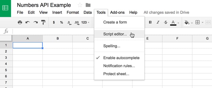
Step 2: Go to the Apps Script editor

Navigate to Tools > Script Editor...

Access script editor through toolbar

Step 3: Name your project

A new tab opens and this is where we’ll write our code. Name the project: Numbers API Example

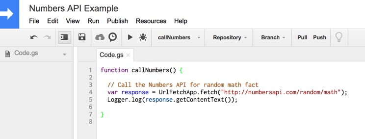
Step 4: Add API example code

Remove all the code that is currently in the Code.gs file, and replace it with this:

function callNumbers() {
  
  // Call the Numbers API for random math fact
  var response = UrlFetchApp.fetch("http://numbersapi.com/random/math");
  Logger.log(response.getContentText());
  
}

We’re using the UrlFetchApp class to communicate with other applications on the internet to access resources, to fetch a URL.

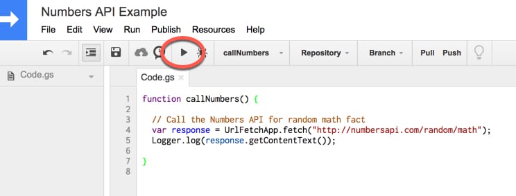
Now your code window should look like this:

Numbers API Google Apps Script code

Step 5: Run your function

Run the function by clicking the play button in the toolbar:

Run Apps Script button

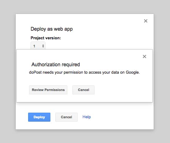
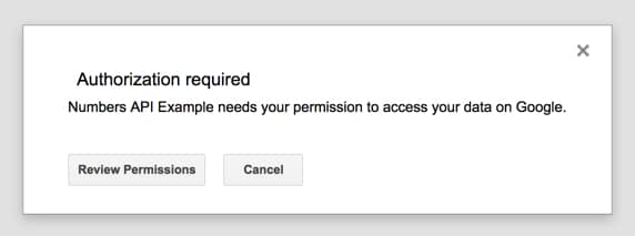
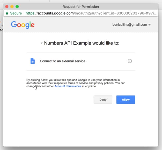
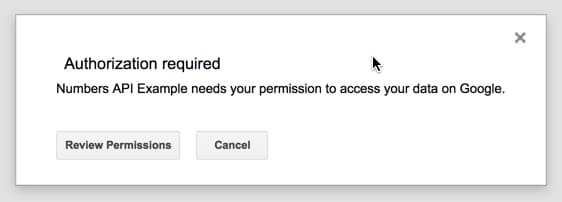
Step 6: Authorize your script

This will prompt you to authorize your script to connect to an external service. Click “Review Permissions” and then “Allow” to continue.

Apps Script Review Permissions

Apps Script authorization

Step 7: View the logs

Congratulations, your program has now run. It’s sent a request to a third party for some data (in this case a random math fact) and that service has responded with that data.

But wait, where is it? How do we see that data?

Well, you’ll notice line 5 of our code above was Logger.log(....) which means that we’ve recorded the response text in our log files.

So let’s check it out.

Go to menu button Execution Log

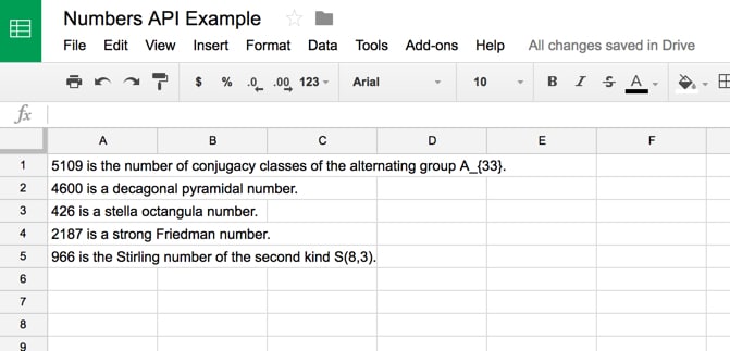
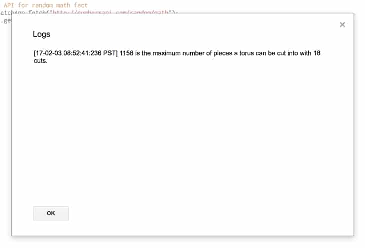
You’ll see your answer (you may of course have a different fact):

[17-02-03 08:52:41:236 PST] 1158 is the maximum number of pieces a torus can be cut into with 18 cuts.

which looks like this in the popup window:

Apps script logger output

Great! Try running it a few times, check the logs and you’ll see different facts.

Next, try changing the URL to these examples to see some different data in the response:

http://numbersapi.com/random/trivia
http://numbersapi.com/4/17/date
http://numbersapi.com/1729

You can also drop these directly into your browser if you want to play around with them. More info at the Numbers API page.

So, what if we want to print the result to our spreadsheet?

Well, that’s pretty easy.

Step 8: Add data to Sheet

Add these few lines of code (lines 7, 8 and 9) underneath your existing code:

function callNumbers() {
  
  // Call the Numbers API for random math fact
  var response = UrlFetchApp.fetch("http://numbersapi.com/random/math");
  Logger.log(response.getContentText());
  
  var fact = response.getContentText();
  var sheet = SpreadsheetApp.getActiveSheet();
  sheet.getRange(1,1).setValue([fact]);
  
}

Line 7 simply assigns the response text (our data) to a variable called fact, so we can refer to it using that name.

Line 8 gets hold of our current active sheet (Sheet1 of Numbers API Example spreadsheet) and assigns it to a variable called sheet, so that we can access it using that name.

Finally in line 9, we get cell A1 (range at 1,1) and set the value in that cell to equal the variable fact, which holds the response text.

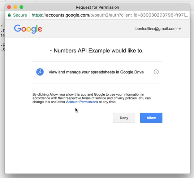
Step 9: Run & re-authorize

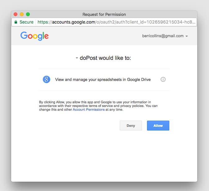
Run your program again. You’ll be prompted to allow your script to view and manage your spreadsheets in Google Drive, so click Allow:

Apps Script Review Permissions

Apps script spreadsheet authorization

Step 10: See external data in your Sheet

You should now get the random fact showing up in your Google Sheet:
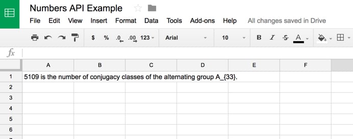
Random math fact from Numbers API in Google Sheet

How cool is that!

To recap our progress so far in this API Tutorial for Beginners: We’ve requested data from a third-party service on the internet. That service has replied with the data we wanted and now we’ve output that into our Google Sheet!

Step 11: Copy data into new cell

The script as it’s written in this API Tutorial for Beginners will always overwrite cell A1 with your new fact every time you run the program. If you want to create a list and keep adding new facts under existing ones, then make this minor change to line 9 of your code (shown below), to write the answer into the first blank row:

function callNumbers() {
  
  // Call the Numbers API for random math fact
  var response = UrlFetchApp.fetch("http://numbersapi.com/random/math");
  Logger.log(response.getContentText());
  
  var fact = response.getContentText();
  var sheet = SpreadsheetApp.getActiveSheet();
  sheet.getRange(sheet.getLastRow() + 1,1).setValue([fact]);
  
}

Your output now will look like this:

Random math facts from Numbers API in Google Sheet

One last thing we might want to do with this application is add a menu to our Google Sheet, so we can run the script from there rather than the script editor window. It’s nice and easy!

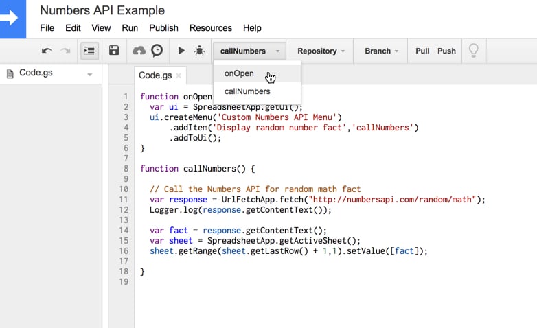
Step 12: Add the code for a custom menu

Add the following code in your script editor:

function onOpen() {
  var ui = SpreadsheetApp.getUi();
  ui.createMenu('Custom Numbers API Menu')
      .addItem('Display random number fact','callNumbers')
      .addToUi();
}

Your final code for the Numbers API script should now match this code on GitHub.

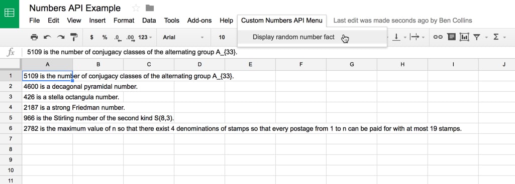
Step 13: Add the custom menu

Run the onOpen function, which will add the menu to the spreadsheet. We only need to do this step once.

Add custom apps script menu

Step 14: Run your script from the custom menu

Use the new menu to run your script from the Google Sheet and watch random facts pop-up in your Google Sheet!

Use custom apps script menu

Alright, ready to try something a little harder?

Let’s build ourselves a music discovery application in Google Sheets.

Example 2: Music Discovery Application using the iTunes API

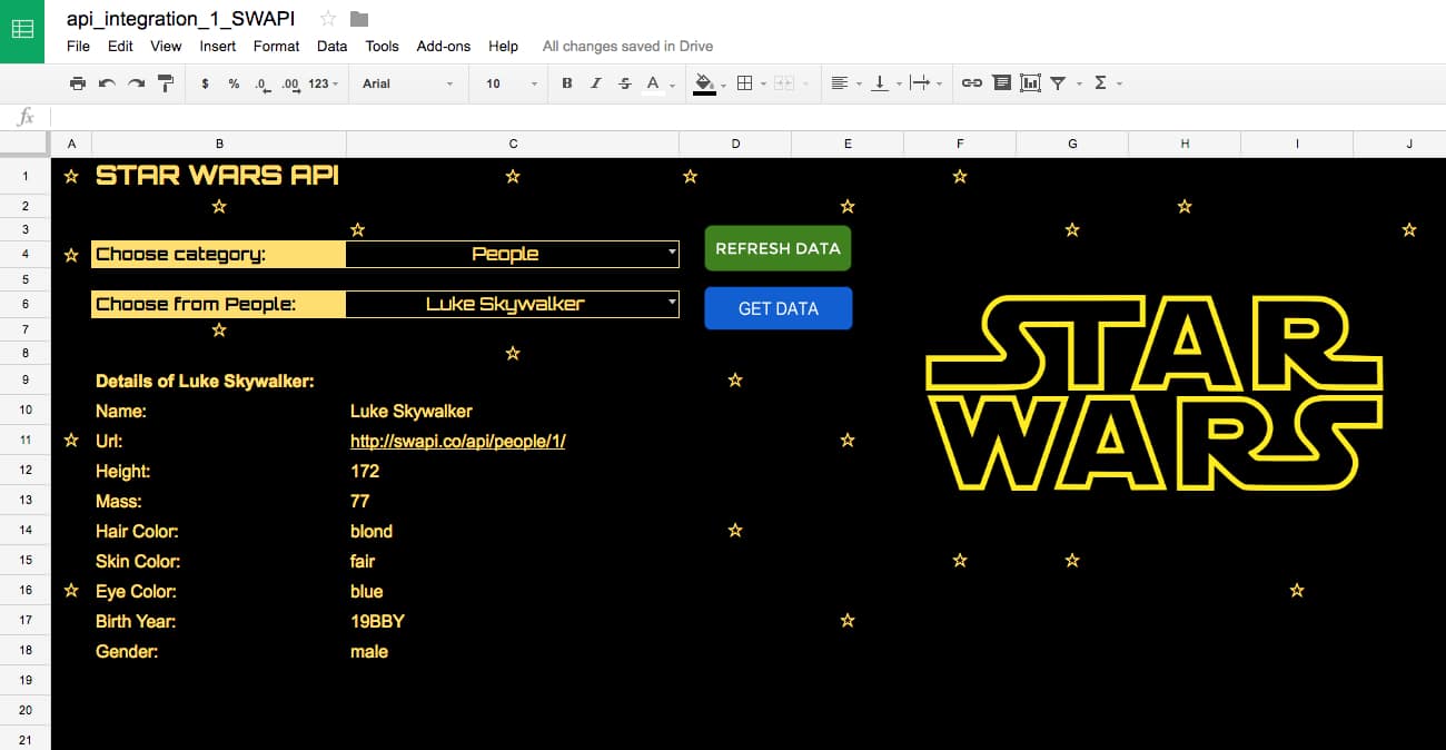
This application retrieves the name of an artist from the Google Sheet, sends a request to the iTunes API to retrieve information about that artist and return it. It then displays the albums, song titles, artwork and even adds a link to sample that track:

Google Sheets and iTunes API using Apps Script

It’s actually not as difficult as it looks.

Getting started with the iTunes API Explorer

Start with a blank Google Sheet, name it “iTunes API Explorer” and open up the Google Apps Script editor.

Clear out the existing Google Apps Script code and paste in this code to start with:

function calliTunes() {
  
  // Call the iTunes API
  var response = UrlFetchApp.fetch("https://itunes.apple.com/search?term=coldplay");
  Logger.log(response.getContentText());
}

Run the program and accept the required permissions. You’ll get an output like this:

iTunes API output

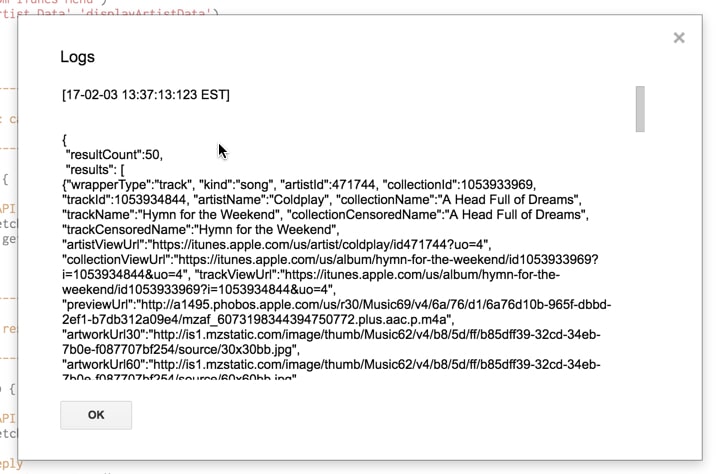
Woah, there’s a lot more data being returned this time so we’re going to need to sift through it to extract the bits we want.

Parsing the iTunes data

So try this. Update your code to parse the data and pull out certain bits of information:

function calliTunes() {
  
  // Call the iTunes API
  var response = UrlFetchApp.fetch("https://itunes.apple.com/search?term=coldplay");
  
  // Parse the JSON reply
  var json = response.getContentText();
  var data = JSON.parse(json);
  
  Logger.log(data);
  Logger.log(data["results"]);
  Logger.log(data["results"][0]);
  Logger.log(data["results"][0]["artistName"]);
  Logger.log(data["results"][0]["collectionName"]);
  Logger.log(data["results"][0]["artworkUrl60"]);
  Logger.log(data["results"][0]["previewUrl"]);
  
}

Line 4: We send a request to the iTunes API to search for Coldplay data. The API responds with that data and we assign it to a variable called response, so we can use that name to refer to it.

Lines 7 and 8: We get the context text out of the response data and then parse the JSON string response to get the native object representation. This allows us to extract out different bits of the data.

So, looking first at the data object (line 10):

iTunes api data packet

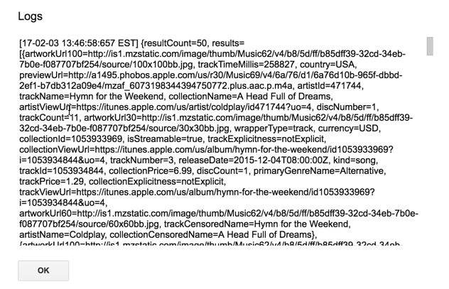
You can see it’s an object with the curly brace at the start {

The structure is like this:

{
resultCount = 50,
results = [ ....the data we're after... ]
}

iTunes api data packet

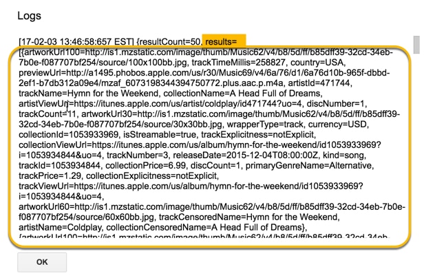
Line 11: we extract the “results”, which is the piece of data that contains the artist and song information, using:

data["results"]

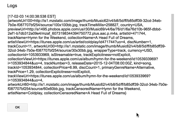
Line 12: There are multiple albums returned for this artist, so we grab the first one using the [0] reference since the index starts from 0:

data["results"][0]

This shows all of the information available from the iTunes API for this particular artist and album:

iTunes api data results

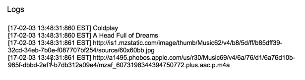
Lines 13 – 16: Within this piece of data, we can extract specific details we want by referring to their names:

e.g. data["results"][0]["collectionName"]

to give the following output:

iTunes api details

Use comments (“//” at the start of a line) to stop the Logger from logging the full data objects if you want. i.e. change lines 10, 11 and 12 to be:

// Logger.log(data);
// Logger.log(data[“results”]);
// Logger.log(data[“results”][0]);

This will make it easier to see the details you’re extracting.

Putting this altogether in an application

If we want to build the application that’s showing in the GIF at the top of this post, then there are a few steps we need to go through:

  • Setup the Google Sheet
  • Retrieve the artist name from the Google Sheet with Google Apps Script
  • Request data from iTunes for this artist with Google Apps Script
  • Parse the response to extract the relevant data object with Google Apps Script
  • Extract the specific details we want (album name, song title, album artwork, preview url)
  • Clear out any previous results in the Google Sheet before showing the new results
  • Display the new results in our Google Sheet
  • Add a custom menu to run the program from the Google Sheet, not the script editor

It’s always a good idea to write out a plan like this before you commit to writing any lines of code.

That way you can think through the whole application and what it’s going to do, which allows you to make efficient choices with how you setup your code.

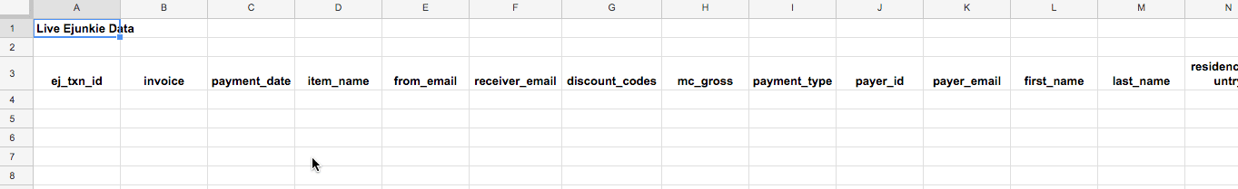
So the first thing to do is setup a Google Sheet. I’ll leave this up to you, but here’s a screenshot of my basic Google Sheet setup:

iTunes Google Sheet

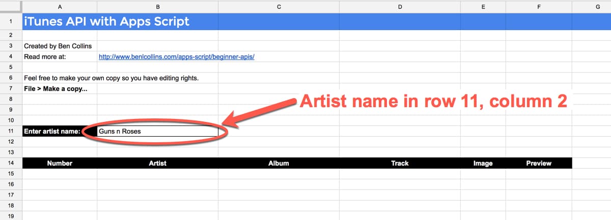
The important thing to note is the location of the cell where a user types in the artist name (11th row, 2nd column) as we’ll be referring to that in our code.

iTunes API Explorer code

And here’s the Google Apps Script code for our application:

// --------------------------------------------------------------------------------------------------
//
// iTunes Music Discovery Application in Google Sheets
//
// --------------------------------------------------------------------------------------------------

// custom menu
function onOpen() {
  var ui = SpreadsheetApp.getUi();
  ui.createMenu('Custom iTunes Menu')
      .addItem('Get Artist Data','displayArtistData')
      .addToUi();
}

// function to call iTunes API
function calliTunesAPI(artist) {
  
  // Call the iTunes API
  var response = UrlFetchApp.fetch("https://itunes.apple.com/search?term=" + artist + "&limit=200");
  
  // Parse the JSON reply
  var json = response.getContentText();
  return JSON.parse(json);
  
}


function displayArtistData() {
  
  // pick up the search term from the Google Sheet
  var ss = SpreadsheetApp.getActiveSpreadsheet();
  var sheet = ss.getActiveSheet();
  
  var artist = sheet.getRange(11,2).getValue();
  
  var tracks = calliTunesAPI(artist);
  
  var results = tracks["results"];
  
  var output = []
  
  results.forEach(function(elem,i) {
    var image = '=image("' + elem["artworkUrl60"] + '",4,60,60)';
    var hyperlink = '=hyperlink("' + elem["previewUrl"] + '","Listen to preview")';
    output.push([elem["artistName"],elem["collectionName"],elem["trackName"],image,hyperlink]);
    sheet.setRowHeight(i+15,65);
  });
  
  // sort by album
  var sortedOutput = output.sort( function(a,b) {
    
    var albumA = (a[1]) ? a[1] : 'Not known';  // in case album name undefined 
    var albumB = (b[1]) ? b[1] : 'Not known';  // in case album name undefined
    
    if (albumA < albumB) { return -1; } else if (albumA > albumB) {
      return 1;
    }
    // names are equal
    return 0;
  });
  
  // adds an index number to the array
  sortedOutput.forEach(function(elem,i) {
    elem.unshift(i + 1);
  });
  
  var len = sortedOutput.length;
  
  // clear any previous content
  sheet.getRange(15,1,500,6).clearContent();
  
  // paste in the values
  sheet.getRange(15,1,len,6).setValues(sortedOutput);
  
  // formatting
  sheet.getRange(15,1,500,6).setVerticalAlignment("middle");
  sheet.getRange(15,5,500,1).setHorizontalAlignment("center");
  sheet.getRange(15,2,len,3).setWrap(true);
  
}

Here’s the iTunes API script file on GitHub.

How it works:

Let’s talk about a few of the key lines of code in this program:

Lines 16 – 25 describe a function that takes an artist name, calls the API with this artist name and then returns the search results from the API. I’ve encapsulated this as a separate function so I can potentially re-use it elsewhere in my program.

The main program starts on line 28.

On line 34, I retrieve the name of the artist that has been entered on the Google Sheet, and we call our API function with this name on line 36.

On lines 42 – 47, I take the results returned by the API, loop over them and pull out just the details I want (artist name, album name, song title, album artwork and preview track). I push all of this into a new array called output.

Next I sort and add an index to the array, although both of these are not mandatory steps.

On line 68, I clear out any previous content in my sheet.

Then on line 71, I paste in the new data, starting at row 15.

Finally, lines 74 – 76 format the newly pasted data, so that the images have space to show properly.

Run the onOpen() function from the script editor once to add the custom menu to your Google Sheet. Then you’ll be able to run your iTunes code from the Google Sheet:

Custom iTunes API menu

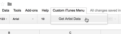
Now you can run the program to search for your favorite artist!

More details on the iTunes API:

Documentation for searching the iTunes Store.

Documentation showing the search results JSON packet.

Example 3: Star Wars data explorer using the Star Wars API

This one is a lot of fun! Definitely the most fun example in this API Tutorial for Beginners.

The Star Wars API is a database of all the films, people, planets, starships, species and vehicles in the Star Wars films. It’s super easy to query and the returned data is very friendly.

Star Wars API in Google Sheet

It’s a little easier than the iTunes API because the data returned is smaller and more manageable, and therefore easier to parse when you first get hold of it.

Getting started with the Star Wars API

As with both the previous APIs, start with a simple call to see what the API returns:

/*
 * Step 1:
 * Most basic call to the API 
 */
function swapi() {
  
  // Call the Star Wars API
  var response = UrlFetchApp.fetch("http://swapi.dev/api/planets/1/");
  Logger.log(response.getContentText());
}

The data returned looks like this:

API Tutorial for Beginners: Star Wars API data

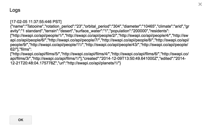
So, it’s relatively easy to get the different pieces of data you want, with code like this:

/*
 * Step 2:
 * Same basic call to the API 
 * Parse the JSON reply
 */
function swapi() {
  
  // Call the Star Wars API
  var response = UrlFetchApp.fetch("http://swapi.dev/api/planets/1/");
  
  // Parse the JSON reply
  var json = response.getContentText();
  var data = JSON.parse(json);
  Logger.log(data);
  Logger.log(data.name);
  Logger.log(data.population);
  Logger.log(data.terrain);
}

Well, that should be enough of a hint for you to give this one a go!

Some other tips

In addition to custom menus to run scripts from your Google Sheet, you can add Google Sheets buttons and connect them to a script to run the script when they are clicked. That’s what I’ve done in this example.

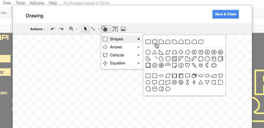
On the menu, Insert > Drawing...

Google Sheets insert drawing

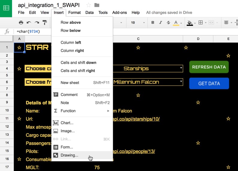
Create a button using the rectangle tool:

Google Sheet drawing tool

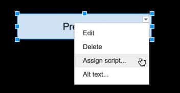
Finally, right click the drawing when it’s showing in your sheet, and choose Assign Script and type in the name of the function you want to run:

Google Sheet drawing assign script

What else?

Use this CHAR formula to add stars to your Google Sheet:

=CHAR(9734)

I used the font “Orbitron” across the whole worksheet and, whilst it’s not a Star Wars font, it still has that space-feel to it.

The big Star Wars logo is simply created by merging a bunch of cells and using the IMAGE() formula with a suitable image from the web.

Finally, here’s my SWAPI script on GitHub if you want to use it.

API Tutorial for Beginners: Other APIs to try

Here are a few other beginner-friendly APIs to experiment with:

> Giphy API. Example search endpoint: Funny cat GIFs

> Pokémon API. Example search endpoint: Pokemon no. 1

> Open Movie Database API. Example search endpoint: Batman movies

> International Space Station Current Location. Example search endpoint: ISS current location

Also, here’s the official Google documentation on connecting to external APIs.

Finally, here’s a syntax guide for the common forms of API Authentication using Apps Script.

Let me know in the comments what you do with all these different APIs!

Disclosure: Some of the links in this post are affiliate links, meaning I’ll get a small commission if you click the link and subsequently signup to use that vendor’s service. I only do this for tools I use myself and wholeheartedly recommend.

Community Connectors: Access all your data in Google Data Studio

Data Studio is relatively new dashboard tool from Google, launched in mid-2016. It’s a superb tool for creating professional looking reports, easily and quickly, and it connects seamlessly to other Google data sources (e.g. Analytics, AdSense, Sheets, …).

Here’s an introduction to Data Studio and a look at the more advanced features.

GitHub commit dashboard, built with the new native data Community Connector
GitHub commits dashboard, built in Data Studio using a native Data Connector

Do you work with data outside of Google’s ecosystem though?

I’ll go out on a limb here, and say, yes, most likely you do.

Perhaps you’re a digital marketing analyst looking at Facebook, Twitter, Instagram, MailChimp data (etc…) for example.

Many of us work with other web services and you want that data displayed in Data Studio. With the launch of native data Community Connectors, you can connect to your favorite web services and access data that lives outside the Google ecosystem directly!

What is a Data Studio Community Connector?

Data Studio Community Connector example
Data Studio Community Connector example with the MailChimp API (click to enlarge)

Continue reading Community Connectors: Access all your data in Google Data Studio

Show data from the GitHub API in Google Sheets, using Apps Script and Oauth

This post shows you how to connect a Google Sheet to GitHub’s API, with Oauth and Apps Script. The goal is to retrieve data and information from GitHub and show it in your Google Sheet, for further analysis and visualization.

If you manage a development team or you’re a technical project manager, then this could be a really useful way of analyzing and visualizing your team’s or project’s coding statistics against goals, such as number of commits, languages, people involved etc. over time.

Contents

  1. What are Git and GitHub?
  2. Access GitHub API using Basic Authentication
  3. Access GitHub API using OAuth2 Authentication
  4. Resources and further reading

Note, this is not a post about integrating your Apps Script environment with GitHub to push/pull your code to GitHub. That’s an entirely different process, covered in detail here by Google Developer Expert Martin Hawksey.

Continue reading Show data from the GitHub API in Google Sheets, using Apps Script and Oauth

How to Create an Annotated Line Graph in Google Sheets

line graph in Google Sheets
Animated line chart in Google Sheets

This post looks at how to make a line graph in Google Sheets, an advanced one with comparison lines and annotations, so the viewer can absorb the maximum amount of insight from a single chart.

For fun, I’ll also show you how to animate this line graph in Google Sheets.

Want your own copy of this line graph?

Click here to access your copy of this template >>

This chart was originally developed for The Write Life during their 4-day product sale earlier this year. It featured as part of a dashboard that was linked to the E-junkie sales platform and displayed sales data in real-time:

Google Sheet e-junkie real-time dashboard

As with any graph, we start with the data:

The data table

Line graph data table

The key to this line graph in Google Sheets is setting up the data table correctly, as this allows you to show an original data series (the grey lines in the animated GIF image), progress series lines (the colored lines in the animated GIF) and current data values (the data label on the series lines in the GIF).

In this example, I have date and times as my row headings, as I’m measuring data across a 4-day period, and sales category figures as column headings, as follows:

Annotated line graph data table

Red columns

The red column, labeled with 1 above, contains historic data from the 2015 sale.

Red column 2 is a copy of the same data but only showing the progress up to a specific point in time.

In red column 3, the following formula will create a copy of the last value in column 2, which is used to add a value label on the chart:

=IF(AND((C2+C3)=C2,C2<>0),C2,"")

Purple columns:

Purple columns 4,5 and 6 are exactly the same but for 2016 data. The formula in this case, in column 6, is:

=IF(AND((F2+F3)=F2,F2<>0),F2,"")

Green columns:

Data in green columns 7 and 8, is our current year data (2017), so in this case there is no column of historic data. The formula in column 8 for this example is:

=IF(AND((H2+H3)=H2,H2<>0),H2,"")

Creating the line graph in Google Sheets

Highlight your whole data table (Ctrl + A if you’re on a PC, or Cmd + A if you’re on a Mac) and select Insert > Chart from the menu.

In the Recommendations tab, you’ll see the line graph we’re after in the top-right of the selection. It shows the different lines and data points, so all that’s left to do is some formatting.

Line graph selection

Format the series lines as follows:

  • For the historic data (columns 1 and 4 in the data table), make light grey and 1px thick
  • For the current data (columns 2, 5 and 7 in the data table), choose colors and make 2px thick
  • For the “max” values (columns 3, 6 and 8 in the data table), match the current data colors, make the data point 7px and add data label values (see steps 1, 2 and 3 in the image below)

Line graph data labels

This is the same technique I’ve written about in more detail in this post:

How can I annotate data points in Google Sheets charts?

Animating the chart with Apps Script

How about creating an animated version of this chart?

Oh, go on then.

When this script runs, it collects the historic data, then adds that data back to each new row after a 10 millisecond delay (achieved with the Utilities.sleep method and the SpreadsheetApp.flush method to apply all pending changes).

I don’t make any changes to the graph or create any fancy script to change it, I leave that up to the Google Chart Tool. It just does its best to keep up with the changing data, although as you can see from the GIF at the top of this post, it’s not silky smooth.

By the way, you can create and modify charts with Apps Script (see this waterfall chart example, or this funnel chart example) or with the Google Chart API (see this animated temperature chart). This may well be a better route to explore to get a smoother animation, but I haven’t tried yet…

Here’s the script:

function startTimedData() {
  var ss = SpreadsheetApp.getActive();
  var sheet = ss.getSheetByName('Animated Chart');
  var lastRow = sheet.getLastRow()-12;
  
  var data2015 = sheet.getRange(13,2,lastRow,1).getValues(); // historic data
  var data2016 = sheet.getRange(13,5,lastRow,1).getValues(); // historic data
  
  // new data that would be inputted into the sheet manually or from API
  var data2017 = [[1],[7],[14],[19],[27],[32],[34],[36],[44],[49],[57],[65],[72],[76],[79],[86],[92],[99],[104],[109],[111],[112],[120],[128],[130],
                  [132],[133],[140],[144],[149],[151],[152],[158],[162],[170],[177],[179],[184],[188],[194],[200],[205],[211],[216],[224],[232],[238],
                  [241],[246],[248],[252],[259],[266],[268],[276],[284],[291],[299],[300],[301],[306],[311],[315],[316],[323],[324]];
  
  for (var i = 0; i &lt; data2015.length;i++) {
    outputData(data2015[i],data2016[i],data2017[i],i);
  }
  
}

function outputData(d1,d2,d3,i) {
  var ss = SpreadsheetApp.getActive();
  var sheet = ss.getSheetByName('Animated Chart');
  
  sheet.getRange(13+i,3).setValue(d1);
  sheet.getRange(13+i,6).setValue(d2);
  sheet.getRange(13+i,8).setValue(d3);
  Utilities.sleep(10);
  SpreadsheetApp.flush();
}

function clearData() {
  var ss = SpreadsheetApp.getActive();
  var sheet = ss.getSheetByName('Animated Chart');
  var lastRow = sheet.getLastRow()-12;
  
  sheet.getRange(13,3,lastRow,1).clear();
  sheet.getRange(13,6,lastRow,1).clear();
  sheet.getRange(13,8,lastRow,1).clear();
  
}

On lines 6 and 7, the script grabs the historic data for 2015 and 2016 respectively. For the contemporary 2017 data, I’ve created an array in my script to hold those values, since they don’t exist in my spreadsheet table.

This code is available here on GitHub.

Finally, add a menu for access from your Google Sheet with the following code:

function onOpen() {
  var ui = SpreadsheetApp.getUi();
  
  ui.createMenu("Timed data")
    .addItem("Start","startTimedData")
    .addItem("Clear","clearData")
    .addToUi();
}

This allows you to run the Start and Clear functions directly from your Google Sheet browser tab, rather than the script editor tab.

That’s it. Hit Start and you should see your chart animate before your eyes:

Animated Apps Script chartAnimated Apps Script chart

If you look closely, you’ll also see the data populating your sheet.

How to build a real-time sales dashboard for E-junkie using Google Sheets and Apps Script

It’s day two of a four day product launch. You’ve worked hard all year to create a fantastic product, test your sales systems and tell the world about this amazing offer. You know you’ve sold 100 products so far, but…

…you don’t know whether your ads are effective, which affiliates are really killing it versus which have forgotten about your launch, or even whether your own emails are converting.

Looking at your sales log only, and having to decipher what’s happened since the last time you looked an hour ago, is like trying to drive in the dark without headlights.

Thankfully there is a better way to track your sales, so you can see your data, get insights about what’s working and what’s not, and immediately act to increase your bottom line.

This post looks at how to build a real-time dashboard for the E-junkie digital sales platform using Google Sheets:

Google Sheet e-junkie real-time dashboard
Google Sheet e-junkie real-time dashboard (fictitious data)
Want your own copy of this dashboard?
Click here to access your copy of this template >>

E-junkie is a digital shopping cart, used for selling digital products and downloads. The system handles the shopping cart mechanics, but does not do any data analytics or visualizations.

You can view a transaction log (i.e. a list of all your sales) but if you want to understand and visualize your sales data, then you’ll need to use another tool to do this. Google Sheets is a perfect tool for that.

You can use a Google Sheet to capture sales data automatically in real-time and use the built-in charts to create an effective dashboard.

You’d be crazy not to have a tracking system set up, to see and understand what’s going on during sales events or product launches. This E-junkie + Google Sheets solution is effective and incredibly cheap ($5/month for E-junkie and Google Sheets is free).

The Write Life ran a Writer’s Bundle sale this year, during the first week of April. It’s a bundled package of outstanding resources for writers, including ebooks and courses, heavily discounted for a short 4-day sales window.

I created a new dashboard for The Write Life team to track sales and affiliates during the entire event. This year’s dashboard was a much improved evolution of the versions built for the Writer’s Bundle sales in 2014 (which, incidentally, was my first blog post on this website!) and 2015.

The biggest improvement this year was to make the dashboard update automatically in real-time.

In previous years, the dashboard was updated every 3 hours when new data was manually added from a download of E-junkie sales data. This time, using Apps Script, I wrote a script and set up E-junkie so that every sale would immediately appear in my Google Sheet dashboard.

So, it truly was a real-time dashboard.

Animated e-junkie sales chart in Google Sheets
Animated chart showing fictitious sales data during a flash sale

The real-time dashboard in Google Sheets

Here’s the final dashboard, annotated to show the different sections:

Annotated Google Sheets dashboard
Annotated Google Sheets dashboard with fictitious data (click to enlarge)

There are too many steps to detail every single one, but I’ll run through how to do the E-junkie integration in detail and then just show the concepts behind the Google Sheet dashboard setup.

How to get data from E-junkie into Google Sheets

New to Apps Script? Check out my primer guide first.

Open up a new Google Sheet and in the code editor (Tools > Script editor…) clear out any existing code and add the following:

function doPost(e) {
  var ss = SpreadsheetApp.getActiveSpreadsheet();
  var sheet = ss.getSheetByName('Sheet1');
  
  if (typeof e !== 'undefined') {
    var data = JSON.stringify(e);
    sheet.getRange(1,1).setValue(data);
    return;
  }
}

Save and then publish it:

Publish > Deploy as a web app...

and set the access to Anyone, even anonymous, as shown in this image:

access Google sheets web app

You’ll be prompted to review permissions:

Apps script review permissions

followed by:

Apps script confirm permissions

Click Allow.

This is a one-time step the first time you publish to the web or run your script.

Now we want to test this code by sending a POST request method to this Sheet’s URL to see if it gets captured.

We’ll use a service called hurl.it to send a test POST request.

Open hurl.it, select the POST option in the first dropdown menu, add the URL of your published sheet into the first text box and, for good measure, add a parameter, like so (click to open large version):

Hurl to test POST request

Click “Launch Request”, head back to your Google Sheet and you should now see some data in cell A1 like this (click to open large version):

POST data in Google Sheet

where the data is something like this (the custom parameter shown in red):

{"parameter":{"testValue":"Ben"},"contextPath":"","contentLength":13,"queryString":null,"parameters":{"testValue":["Ben"]},"postData":{"type":"application/x-www-form-urlencoded","length":13,"contents":"testValue=Ben","name":"postData"}}

Voila! The data sent by the POST action is sitting pretty in our Google Sheet!

It’s essentially exactly the same mechanics for the E-junkie example.

So now we know it’s working, let’s change the Sheet and the code to handle E-junkie data.

For the Sheet: Delete the data in cell A1, and add a row of headings that match the headings in lines 12 to 33 of the code below (omitting the data.):

E-junkie Google Sheet set-up

(This screenshot doesn’t show all the columns, some are off-screen to the right.)

For the code: Delete all the previous code and replace with this (note that I’m still referring to Sheet1, so if you’ve changed the name of your Sheet to something else you’ll need to change it in the code on line 4 as well):

function doPost(e) {
  
  var ss= SpreadsheetApp.openById("&lt;Sheet ID&gt;");
  var sheet = ss.getSheetByName("Sheet1");
  
  var outputArray = [];
  
  if(typeof e !== 'undefined') {
    var data = e.parameter;
    
    outputArray.push(
      data.ej_txn_id,
      data.invoice,
      data.payment_date,
      data.item_name,
      data.from_email,
      data.receiver_email,
      data.discount_codes,
      data.mc_gross,
      data.payment_type,
      data.payer_id,
      data.payer_email,
      data.first_name,
      data.last_name,
      data.residence_country,
      data.payer_status,
      data.payment_status,
      data.payment_gross,
      data.affiliate_id,
      data.item_affiliate_fee_total,
      data.mc_currency,
      data.payer_business_name,
      data.payment_fee
    );
    
    sheet.appendRow(outputArray);
  }
  
  return;
}

Here’s the e-junkie code on GitHub.

Save your code and update the published web app (Publish > Deploy as a web app… and click Update).

Copy this updated application URL to your clipboard. Log in to E-junkie and navigate to Edit Preferences:

E-junkie menu

Paste in your URL into the Custom/Third-Party Integration Common Notification URL text box:

E-junkie custom integration

And that’s it!

Whenever you make a sale through E-junkie, you should now see the data show up in your Sheet.

Further reading on the E-junkie integration: Official E-junkie integration documentation

Thanks:

Thanks to Google Developer Expert Riël Notermans who pointed out how to fix the redirect issue I was dealing with in earlier versions of the script.

Thanks to all the kind folks on Stack Overflow who helped me get this working.

Build Business Dashboards With Google Sheets

Digital marketing dashboard in Google Sheets
Learn how to build beautiful, interactive dashboards in my online course.
9+ hours of video content, lifetime access and copies of all the finished dashboard templates.
Learn more

How I created the dashboard in Google Sheets with E-junkie data

Really the crux of this whole example was getting the E-junkie data into my Google Sheet in real-time. Once I had that up and running, I was free to do anything I wanted with the data.

Data staging

The E-junkie sales data looked like this in my Google Sheet once the transactions started to come in (blurred to hide details):

E junkie data

From this raw data, I created a staging table for the line tracking chart:

staging table for line chart

This table was driven by checking whether the hour date in column E of the current row (green) was less than the current time and then counting sales up to that point. The 2014 and 2015 datasets were included for reference.

The extra columns J, K and M were created for the chart annotations (see how to create an annotated line graph in Google Sheets).

To ensure everything updated in near real-time, I changed the calculation settings (File > Spreadsheet settings... > Calculation) to: On change and every minute

Progress tracking chart

The line tracking chart showed progress during the sale period, against the 2014 and 2015 benchmarks.

In action, it looked like this (showing fictitious data, and sped up to show progress through the sale period):

Animated Apps Script chartAnimated Apps Script chart
Read more about how the progress tracking line chart was created (including animation) here.

Revenue/profit bar chart

The revenue/profit chart was a standard bar chart showing total revenue and total profits against the target metrics (fictitious numbers):

Revenue and Profit bar chart

Sales channel metrics

The lower portion of the chart was a breakout of all the different sales channels we tracked, everything from individual emails, to ads (Facebook and Pinterest) and different affiliates.

Every one of these channels had their own row, showing the actual sales performance against that channel’s projected sales (click to view larger version; numbers are fictitious):

Example of sales data

The key formula driving this section of the dashboard was a simple COUNTIF formula, labeled 1 above, which counted the number of sales in the E-junkie dataset attributed to this channel:

=COUNTIF('ejunkie staging data'!$S$4:$S,D25)

The sparkline formula for the green bar charts, labeled 2 above, was:

=IF(J25=0,"",SPARKLINE(J25,{"charttype","bar";"max",MAX($G$25:$G$36);"color1","#4caf50"}))

Note: both of these formulas work for the data in row 25.

In action

One fun thing we did with the dashboard this time around, which I’d never done previously, was to show it full screen on a big TV during the sale, using an Apple TV and AirPlay:

Google Sheet e-junkie dashboard on big screen

Cool! 🙂