Have you ever wished the VLOOKUP function could return multiple columns?
For example, maybe you want to return several values that match a search term so that you can use a range of data as an input for another formula (e.g. a sparkline).
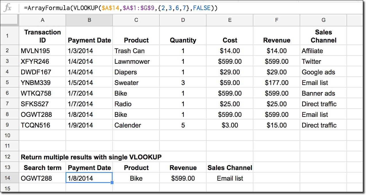
Of course, you could set up multiple vlookup formulas, but this wouldn’t work if you want to pass the data range into another formula, like the sparkline for example.
However, you can easily achieve it with just one formula.
Vlookup return multiple columns
We use array literals {} to indicate which columns we want to return and then convert the formula into an Array Formula to tell Google Sheets we’re working with a range output, not a single value.
What’s the formula to have Vlookup return multiple values?
Assuming I have a data table in range A1:G9 and my search value in A14, as shown in the image above, then the lookup formula is as follows:
=ArrayFormula(VLOOKUP($A$14,$A$1:$G$9,{2,3,6,7},FALSE))Can I see an example worksheet?
How does this formula work?
Imagine this is your raw data table and you want to search for an ID and return values from multiple columns:
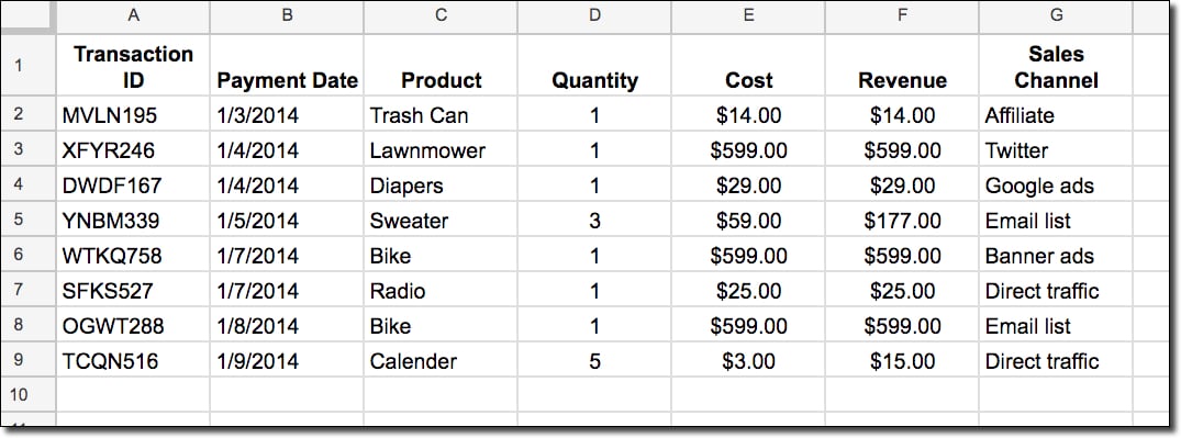
Essentially, we perform a regular VLOOKUP but in place of single column index, we put an array of columns we want to return, surrounded by curly brackets, like so:
{2,3,6,7}
which returns the 2nd, 3rd, 6th, and 7th columns.
Then we must press Ctrl + Shift + Enter (on PC) or Cmd + Shift + Enter (on Mac) once we’ve entered the VLOOKUP to turn it into an array formula. (You can also just type in the ArrayFormula word.)
So we go from this formula:
=VLOOKUP($A$14,$A$1:$G$9,{2,3,6,7},FALSE)which will not work, to this one:
=ArrayFormula(VLOOKUP($A$14,$A$1:$G$9,{2,3,6,7},FALSE))which does work and will output an array (i.e. multiple values). It’s important that the output cells (4 in this case) are all empty for the formula to work.
This is what’s happening:

We search for a single search term and return values from four columns which are output into for adjacent cells. You can select whichever columns you wish as well as changing the order.

That was very helpful. Thank you!
Ben, Given your example above, is it possible to sort the results by column 6?
Thank you for your site and videos….they’ve been an invaluable resource to help me learn!
Perhaps wrap in QUERY(…, “select * order by Col3 desc”) where Col3 refers to the column that would be returned by your ArrayFormula upon which you wish to sort. It does not relate to the original column name.
Hi
I wanted to test this but it is not working for me.
First question,
why is your seperator in the formula a ,
i have to use a ;
then if i use your sheet the formular is working but if i copy all content from your sheet in a new sheet and then try to get the formular to work it will not.
and you write Ctrl + Shift + Enter but nothing happens for me ?
Hi Kijan, if you’re based in Europe, then there are syntax differences in formulas, which I explain here: https://www.benlcollins.com/spreadsheets/sheets-location/
You can add array formulas manually by typing ArrayFormula( at the beginning of your formula.
Cheers,
Ben
I had the same problem, and I was puzzled why before I could use this formula without any problem, and what happened that it stopped working when implementing in other sheets. Then it turned out that somehow this range inside the {} should still be , though you use a locale that requires ; as formula separator.
Finally I made it work by tweaking the formula a bit in this way:
=ArrayFormula(VLOOKUP($A$14,$A$1:$G$9,transpose({2;3;6;7}),FALSE))
Only later on I figured out what Ben showed in the link he gave about the differences in the syntax, that instead of , for line separator you have to use \ and then the formula should look like so:
=ArrayFormula(VLOOKUP($A$14,$A$1:$G$9,{2\3\6\7},FALSE))
Thanks!! 🙂
That solved my problem too!
The “\” part, with “;” it was picking a column for each row!
Is it possible to make the column index dynamic. For example, If my formula was =VLOOKUP(Named Range 1, ImportXML Range 2,{2,3,4,5},False) but I wanted to automatically add the next column in sequence with a dynamic reference, could it be done? Ive played around with Jointext and Split and Sequence but cant get it to work like it does with dynamic columns in Query.
Hello,
Is it possible to use something similar to this to get the column outputs as described for all occurances of the input in a given column? In other words, in the example above you have just one entry of “OGWT288” in column A. What if you have potentially more entries of your trigger input in column A? For example, if you were a hotel getting ready to pay travel agent commissions, and your commission eligible transaction data was in good shape, could you use something similar to find each instance of a given inputted IATA number, and return the wanted column data for each instance, not just for the first match of the IATA number found?
If this isn’t the right tool for the task, would you be so kind as to point me in the right general direction? I’m fairly resourceful, but I am not yet understanding how to get returns beyond the first match. Any advice? Thank you very kindly.
Thank you for this awesome tip!
When you use Arrayformula you can name the column
Example: ={“Date of Birth”;array_constrain(arrayformula(text(VLOOKUP($C$2:C,DataPHX!$A$2:$B,2),”mmm-dd”)),counta($C$2:$C),1)}
This return “Date of Birth” at the top of the column.
I was wondering whether you can name each column when using this tip. How would I name the following columns “Gender”, “Nationality”, “Phone Number” etc:
=ARRAYFORMULA(vlookup($C$2:$C,Data2!$A$3:$AF$2244,{23,24,31,32,20,26},False))
Thank you in advance
What is very taxing: (a) this approach using vlookup+array literals (say, input in one cell, output 5 cells), or (b) the usual arrayformula+vlookup (say, input formula in each 5 cells)?
Great approach. I just used the lazy way by joining the columns into one then splitting them back out haha