GETPIVOTDATA Function in Google Sheets: How To Extract Data From Pivot Tables

The GETPIVOTDATA function is used to extract data from a pivot table.

Pivot tables are one of the most powerful and useful features in spreadsheets. We use them to summarize our data, by grouping, sorting and filtering it.

But pivot tables are dynamic elements. That means they can change size and shape when data is added or removed from the underlying dataset (e.g. when a new category is added). This makes it tricky to extract data consistently.

When a pivot table changes size, a regular cell reference (e.g. A12 or F34) might not point to the correct value in the pivot table anymore. However, the GETPIVOTDATA function will still extract the correct data.

The downside of GETPIVOTDATA is that it’s fiendishly difficult to use. It’s something of a dark art to identify the correct rows and columns inside the function.

In this post, we’re going to learn how this function works.

👇 Feel free to grab the template from the bottom of this article to follow along.

Our Dataset

Let’s use this simple dataset for this tutorial, showing exam scores for 4th – 6th graders in various subjects. It’s presented using the new Tables feature in Google Sheets:

Example 1: GETPIVOTDATA for total values

Now, let’s create a pivot table from this dataset.

Select a cell anywhere inside the dataset.

Then go to the menu Insert > Pivot table

Click “Create”. (You can create the pivot table in a new Sheet or, as I’ve done in this example, in the existing Sheet, next to the data table.)

Here’s our pivot table:

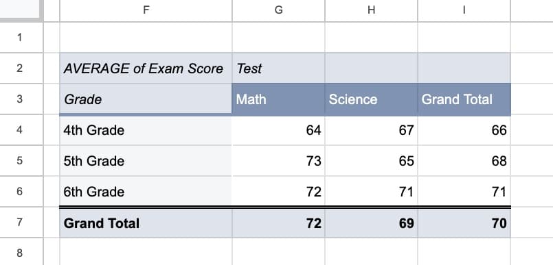
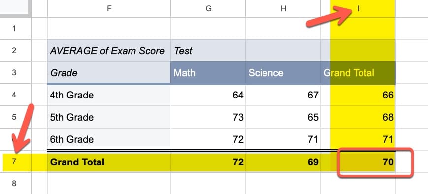
Suppose we want to grab that Grand Total value from cell I7 and display it or use it somewhere else in our Sheet. Perhaps we want to include the value on our dashboard or in a report Sheet.

We might try this formula

=I7

which would work fine provided the pivot table remains static.

But, if new data is added to our dataset then it changes the size of the pivot table.

In our example, let’s add two new rows to the original dataset, with a new grade (“7th Grade”) and test (“Geography”) categories:

(Compare this with the original dataset at the top of this post.)

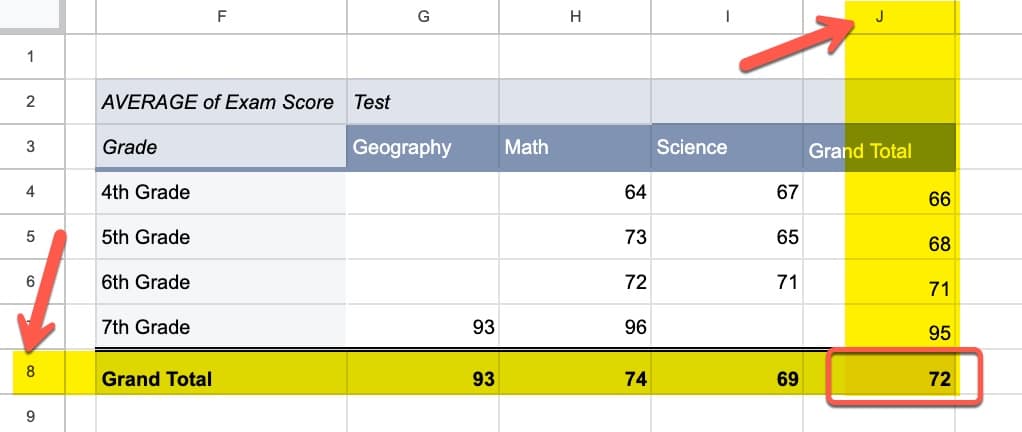
The pivot table has expanded to include an extra row and column for these new categories (“7th Grade” and “Geography”).

So the original I7 formula no longer picks up the correct value.

Cell I7 is now blank and the grand total is now in cell J8:

To fix this, let’s use the GETPIVOTDATA function. This formula ensures we get the total value, even if the pivot table updates:

AVERAGE of Exam Score is the name of the value field in our pivot table, which shows in the top left cell of the pivot table. It comes from the value section of the pivot table:

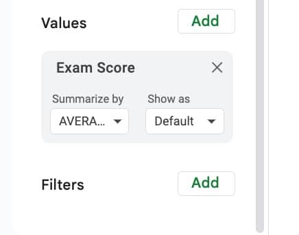
The name in the GETPIVOTDATA formula matches the name from the pivot table.

We selected “Exam Score” as the value in our pivot table and chose to summarize by “AVERAGE”. Therefore, the name for the formula is “AVERAGE of Exam Score”. If we’d chosen “COUNT” instead, then it would be “COUNT of Exam Score”.

F2 is a reference to the top left cell of the pivot table.

Now we’ve seen an example, let’s take a look at the complete function syntax.

GETPIVOTDATA Syntax

The function takes the form:

It takes a minimum of two arguments: value_name and any_pivot_table_cell

value_name

is the name of the value field from the pivot table, enclosed in quotation marks.

any_pivot_table_cell

is a reference to any cell within the pivot table (top left recommended).

In addition, GETPIVOTDATA can have optional pairs of column names and pivot items.

original_column

The name (heading) of a column in the original dataset.

pivot_item

The name of the item we want to retrieve data about, which is found in the pivot table and the original dataset.

Notes

• Arguments are not case-sensitive, except field names.
• If you use a custom heading for a field in your pivot table, use that custom heading in your GETPIVOTDATA formula instead of the column name from the source data.

Example 2: extract a column total

If we want a column total (e.g. the Science column) rather than the grand total, we need to specify that in our formula.

We do that by referencing the column name in the underlying data set!

In the underlying dataset, I have a column called “Test”, which we refer to inside of the formula:

The following image shows the formula highlighted in cell G12:

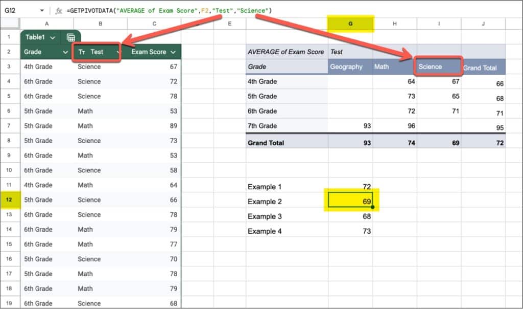
The red arrows illustrate how GETPIVOTDATA formula refers back to the “Test” column in the original dataset. And within Test, we’re interested in “Science”.

Example 3: extract a row total with GETPIVOTDATA

Similarly, to get a row total from our pivot table, we reference the name from the underlying dataset.

To get the row total for “5th Grade”, we have this formula in cell G13:

Shown in the Sheet:

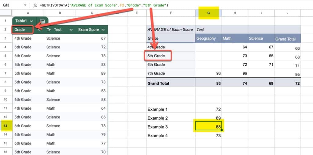
The red arrows show how the GETPIVOTDATA formula refers back to the column in the underlying dataset.

Example 4: extract a specific value

To get a specific value in the pivot table, at the intersection of a row and column, e.g. 5th Grade and Science, we have to specify both conditions with reference to… you guessed it, the underlying data columns:

Shown in the Sheet:

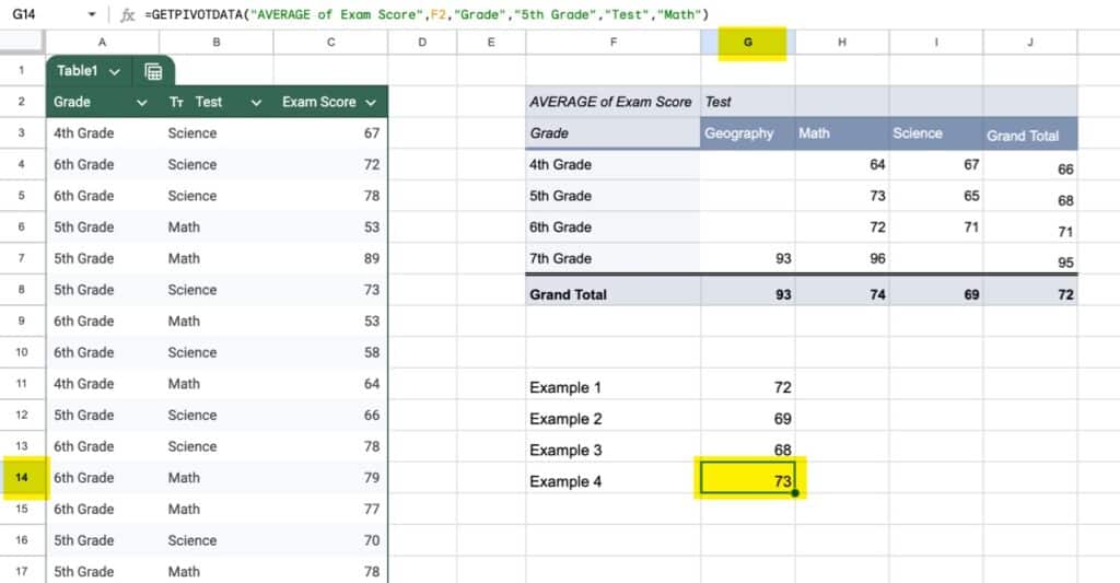
There are too many columns to show with red arrows in this image, but look for the column names from the original dataset in the GETPIVOTDATA formula.

GETPIVOTDATA Template

Click here to open a view-only copy >>

Feel free to make a copy: File > Make a copy…

If you can’t access the template, it might be because of your organization’s Google Workspace settings. If you click the link and open in an Incognito window you’ll be able to see it.

The IF function is also covered in the Day 28 lesson of my free Advanced Formulas 30 Day Challenge course.

You can also read about it in the Google documentation.

Writing this tutorial has made GETPIVOTDATA feel a little less like black magic to me. Hopefully for you too.