Whether you’re just starting out with Google Sheets or are a seasoned pro, sooner or later one of your formulas will give you a formula parse error message rather than the result you want.
It can be frustrating, especially if it’s a longer formula where the formula parse error may not be obvious.
In this post, I’ll explain what a Google Sheets formula parse error is, how to identify what’s causing the problem, and how to fix it.
What is a formula parse error?
Before we get into the different types of errors, you might be wondering what does formula parse error mean?
Essentially, it means Google Sheets can’t interpret your formula. It can’t fulfill the formula request so it returns an error message.
There are a variety of ways this can happen — everything from typos to mathematical impossibilities — and we’ll explore them all in detail below.
Understanding the meaning behind the error messages, and learning how to fix them, is a crucial step to becoming a formula pro in Google Sheets.
Auditing and Debugging Formula Parse Errors in Google Sheets
Match the error message in your Google Sheet to the sections below, and find out what might be causing your error.
- An formula parse error message popup prevents me entering my formula
- I’m getting an #N/A error message
- I’m getting an #DIV/0! error message
- I’m getting an #VALUE! error message
- I’m getting an #REF! error message
- I’m getting an #NAME? error message
- I’m getting an #NUM! error message
- I’m getting an #ERROR! error message
- I’m getting an #NULL! error message
- Other strategies for dealing with errors
- Functions to help deal with formula errors in Google Sheets
- Help! My formula is STILL not working
Here’s a Google Sheet with all these examples in.
1. A formula parse error message popup prevents me entering my formula
You think you’ve finished your formula, so you hit enter and boom! You get slapped with a popup message box "Houston, we have a problem" or similar:
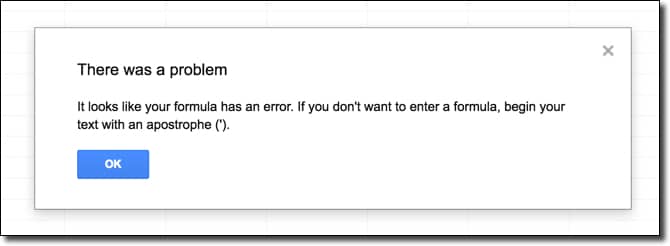
It’s reasonably rare that you’ll experience this, and it usually points to some fundamental problem with your formula.
For example, imagine that as you hit the Enter key, you also accidentally struck the “\” key (which is right above the Enter key) and inadvertently added that to the end of your formula:
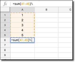
This will result in the popup error message. It’s easily corrected by removing the unwanted character.
How to correct this error?
Try to avoid these in the first place by checking your formula prior to hitting enter. Make sure you’re not missing a cell reference and you don’t have any unwanted characters lurking.
2. I’m getting an #N/A error message. How do I fix it?
The #N/A formula parse error signifies that a value is not available.
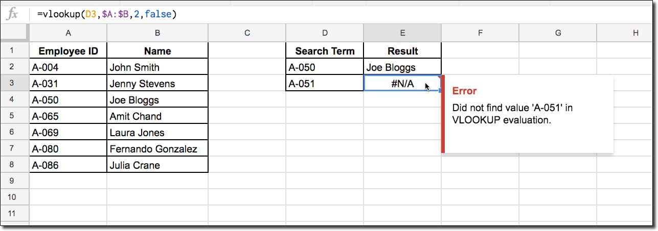
It happens most frequently when you’re using a lookup function (e.g. the VLOOKUP function) and the search term isn’t found. This is exactly what has happened in the exact match VLOOKUP in the image above. The search term A-051 is not in our data table so the formula returns #N/A.
This formula is not wrong or broken, so we don’t want to delete it. However, it would be cool if you could display a custom message, something like “Result not found”, instead of #N/A error message, especially if you have a lot of these errors showing. It gives the spreadsheet user much more information and reduces confusion.
Thankfully we can:
How to correct an #N/A error?
Well, there’s this super handy IFERROR function in Google Sheets:
In this VLOOKUP example, the full formula would look like this:
as shown in this example:
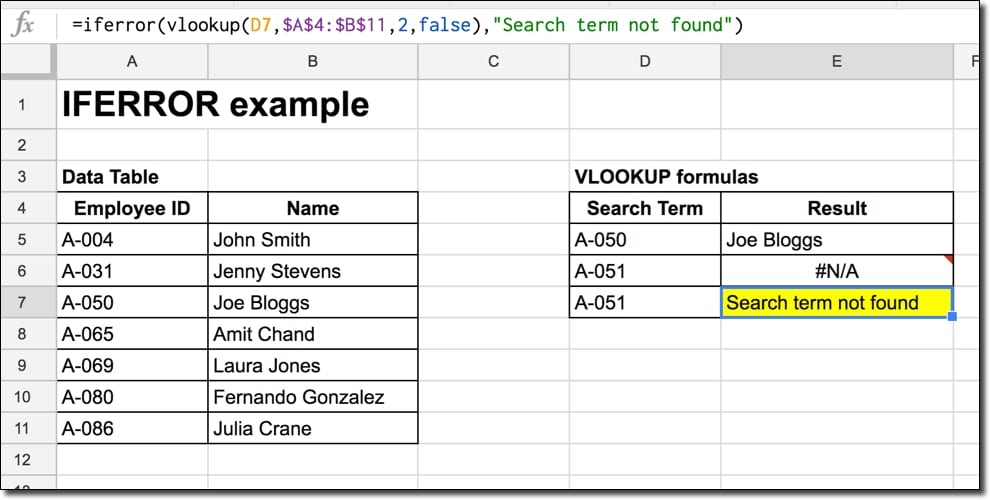
Instead of showing the #N/A formula parse error when a value is not found, the formula will output our custom message instead “Search term not found”.
3. I’m getting an #DIV/0! error message
This formula parse error happens when a number is divided by zero, which can occur when you have a zero or a blank cell reference in the denominator.
In layman’s terms, what this means is that we’re trying to compute something like this:
= A / 0which has no meaning because you can’t divide by 0.
Read more about division by 0 here, although it gets super technical super quickly.
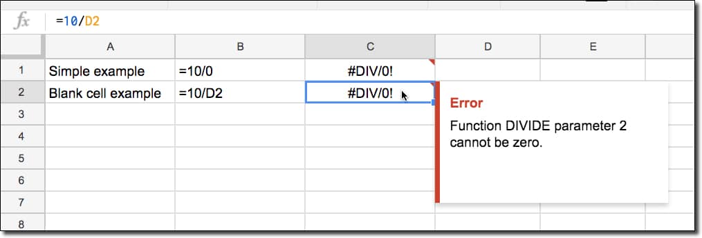
Another example is using a formula like AVERAGE with a blank range.
= AVERAGE(A1:A10)will cause a #DIV/0! error if the range A1:A10 contains no numerical values.
How to correct an #DIV/0! error?
Well, the first thing to do is determine why your denominator is evaluating to zero.
You can select the denominator and see what it is evaluating to by highlighting it in the formula bar, and seeing what the result is in the little popup box, as shown in this image:
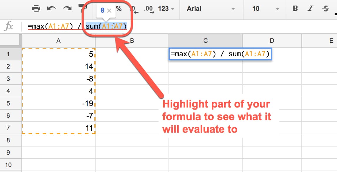
In this case, the formula in the denominator SUM(A1:A7) evaluates to 0, which causes the error. So check whether your denominator result is 0.
Next, check whether you have linked to blank cells or a blank range in your denominator. Then you can either fill in the blank cell or range, or select a different cell or range for your formula.
If your formula is correct and your cell/ranges are not unintentionally blank, then you’ll want to handle the #DIV/0! error. It looks unsightly and makes your spreadsheet look unfinished if you leave these errors floating around.
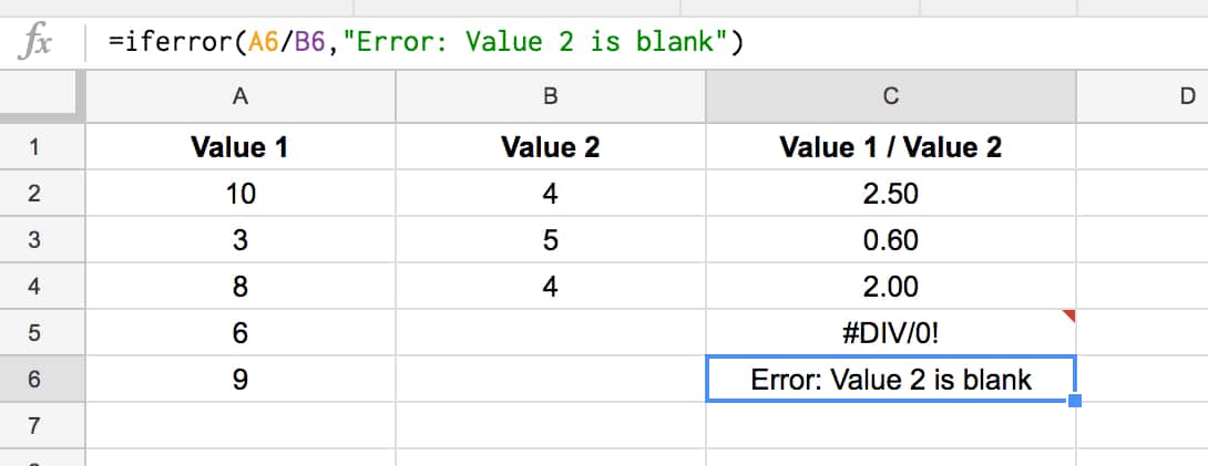
As with the #N/A error example, use the IFERROR formula to wrap your current formula and specify a result for when a #DIV/0! error occurs. You might want to output an error message, e.g. “Division by 0 error”, or maybe a specific value, e.g. 0:
4. I’m getting an #VALUE! error message
This formula parse error typically occurs when your formula is expecting a certain data type as an input but receives the wrong type, for example trying to do math operations on a text value instead of a numerical value.
Spaces in your cells can also cause this error message.
In this example, cell B1 contains a space, which is a string value and causes the #VALUE! error because Google Sheets can’t perform a math operation on it, as seen in this error message:
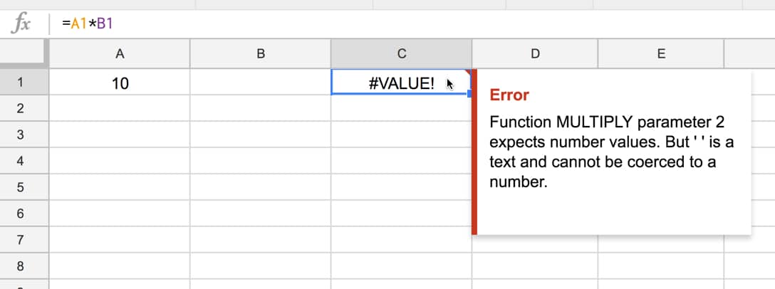
In general, Google Sheets do a pretty good job of coercing text into numbers when needed. If you enter a value into a cell with some spaces, format it as text and then try to do math on it, Google Sheets will actually force the text into a number and still perform the calculation.
Another cause of #VALUE! errors is mixing US and Rest of World date formats.
US dates have the form MM/DD/YYYY whilst the Rest of the World goes for DD/MM/YYYY. If you have a mix of the two and try to subtract them to get the number of days between them for example, you’ll get the #VALUE! error.
(In fact, it’s the same text/number issue happening underneath the surface. Dates are stored as numbers, but if you’re date is in the wrong format for the country setting for your spreadsheet, it’ll be stored as a text string and Google won’t know it’s meant to be a date.)
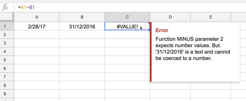
Here the correct answer should have been 59, the number of days between the 28 Feb 2017 and the 31st Dec 2016.
How to correct an #VALUE! error?
The error message should give you some information on which part of your formula is causing the problem.
Search for any possible text/number mismatches, or cells containing errant spaces. If you click into a cell and the flashing cursor has a gap between itself and the element it’s next to, then you’ll have a space there.
Cells can look empty but still contain spaces:
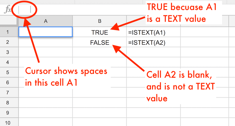
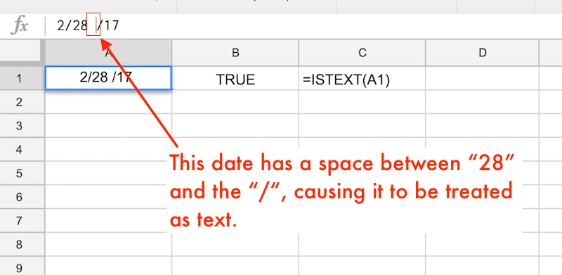
Dates with spaces in the middle won’t work either:
5. I’m getting a #REF! error message
The #REF! formula parse error occurs when you have an invalid reference.
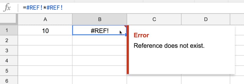
Missing reference: For example when you reference a cell in your formula that has since been deleted (not the value inside the cell, but the whole cell has been deleted, typically when you’ve deleted a row or column in your worksheet).
In this example, the original formula was
= A1 * B1but when I deleted column A, the formula went haywire because of the missing reference:
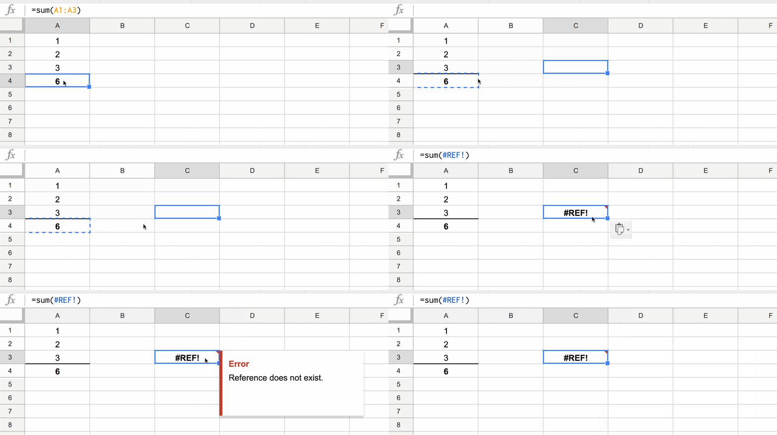
Another way that a formula can refer to missing references is when you copy a formula with a relative range at the edge of your sheet. When you copy and paste, it’s possible the relative range moves as if it were outside the bounds of the sheet, which is not allowed and will cause a #REF! error.
In this example, the sum function adds the cells in the 3 rows above. When I try to copy-paste the sum function into a new cell with fewer than 3 rows above, it’ll give me the #REF! error:
Lookup out of bounds: You’ve probably seen the #REF! error if you use lookup formulas frequently, when you’ve tried to return a value outside of ranges you’ve specified. In this VLOOKUP example, I’m trying to return an answer from the 3rd column of a search table that only has 2 columns:

Circular dependency: You’ll also get a #REF! error when a circular dependency is detected (when the formula refers to itself).
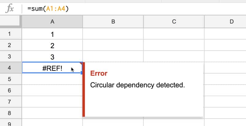
In this example, I have numbers in the range A1 to A3, but the SUM formula in cell A4 tries to sum from A1 to A4, which includes itself. Hence, we have a circular argument where cell A4 is trying to be both an input and output cell, which is not allowed.
How to correct a #REF! error?
First of all, read the error message to determine what kind of #REF! error you’re dealing with. This should give you a big hint on how to correct the error.
For deleted references, look for the #REF! error is inside your formula, and replace the #REF! with the correct reference to a cell or range.
For out-of-bound lookup errors, look through your formula carefully and check your range sizes against any row or column indexes you’re using.
For circular dependencies, find the reference that’s causing the problem (i.e. where you refer to the current cell inside your formula too) and modify it.
6. I’m getting a #NAME? error message
The #NAME? formula parse error signifies a problem with your formula syntax.
The most common reason for this error is a misspelling in one of your function names.
In this example, I misspelt the SUM function as SUMM, which Google Sheets didn’t recognize, so returned an error:
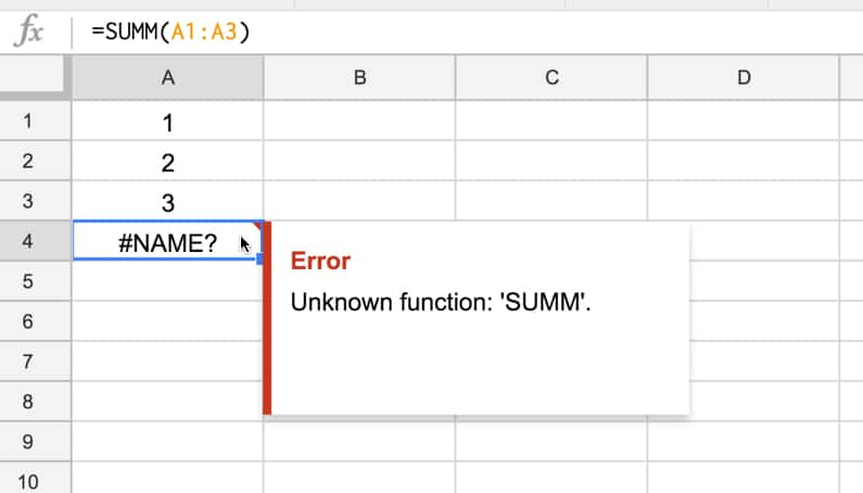
Another reason for a #NAME? error is referencing a named range that doesn’t actually exist or is misspelled.
So
=SUM(profit)will give you a #NAME? error if the named range profit does not exist
Missing quotation marks around a text value, as shown in this simple formula, will also cause a #NAME? error:
=CONCAT("First",Second)(The word Second is missing quotation marks.)
How to correct an #NAME? error?
Check your function names are correct. Use the function helper wizard to reduce the chances of errors happening, especially for the functions with longer names. As you start typing your formula, you’ll see a menu of functions, which you can select with the up and down arrows and Tab.
Check you have defined all named ranges before using them in your formulas and that they all have the correct spellings.
Check any text values are entered with the required quotation marks.
Lastly, have you missed the colon in your range references? It’ll be obvious because it won’t be highlighted correctly.
This formula
=SUM(A1A10)is missing the colon between A1 and A10 and will throw a #NAME? error.
It should of course read:
=SUM(A1:A10)7. I’m getting an #NUM! error message
The #NUM! formula parse error is shown when your formula contains numeric values that aren’t valid.
The classic example is trying to find the square root of a negative number, which isn’t allowed:
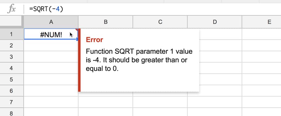
(For any math geeks out there, you’ll know that you can resolve square roots of negative numbers with complex (imaginary) numbers.)
Some other functions that can result in #NUM! error messages are the SMALL function and LARGE function. If you try to find the smallest n-th value in your dataset, where n is outside the count of values in your dataset, you’ll get a #NUM! error.
For example, you ask Google Sheets to find the 10th smallest number in a dataset that only has 5 values in it:
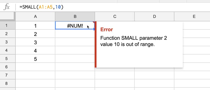
(Why this doesn’t return a #REF! error like the VLOOKUP out of bounds example, I don’t know.)
How to correct a #NUM! error?
You need to check the numeric arguments in your formula. The error message should give you some hints about which part of the formula is causing the issue.
8. I’m getting an #ERROR! formula parse error message
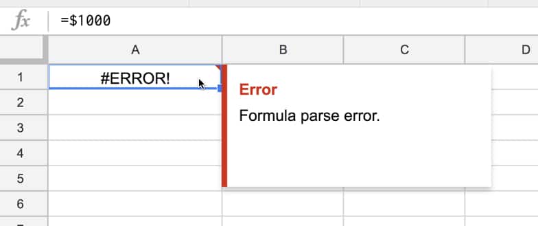
This formula parse error message is unique to Google Sheets and doesn’t have a direct equivalent in Excel. It means that Google Sheets can’t understand the formula you’ve entered, because it can’t parse the formula to execute it.
For example, if you manually type in a $ symbol to refer to an amount, but Google Sheets thinks you’re referring to an absolute reference:
or you’ve missed a “&” when concatenating text and numerical values:
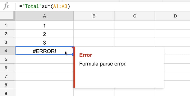
In this case the formula should be:
="Total "&sum(A1:A3) Another case, caused when we messed up the closing brackets of a formula:
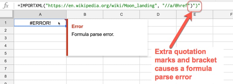
How to correct an #ERROR! error?
Carefully check your formula for accuracy.
You want to ensure you’ve got the correct number of brackets and correct join syntax between text and numerical values (e.g. using “&”).
When you want to show values with currency symbols or as percentages, don’t manually type in the “$” or the “%”. Instead, enter a plain number and then use the formatting options to change it to the style you want.
9. I’m getting an #NULL! error message
I haven’t been able to recreate a #NULL! formula parse error in the wild but theoretically, it exists!
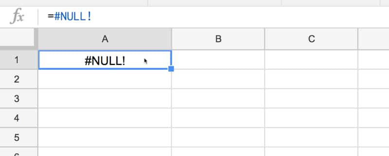
(If you have one showing in your sheet, let me know! I’d love to update this article with an example here.)
10. Other strategies for dealing with a formula parse error
Look for red highlighting in your formula as this will help identify the source of your error e.g. in the case of too many brackets, the extra, superfluous ones will be highlighted in red.
Peeling back the onion: the onion framework is a technique to debug errors for long, complex formulas. Unwrap the outer functions in your formula one-by-one, until you get it working again. Then you can start to add them back one-by-one again, and see exactly which step is causing the issue and fix that.
Different syntax in different countries: Some European countries will use semi-colons “;” in place of commas “,” so this could be a cause of your error. Compare these two formula, which have identical inputs and outputs, but the syntax is different for users in different countries (locales).
is the same formula as this:
(This is an example of a VLOOKUP returning multiple values (an array) instead of just a single value.)
Pro tip:
Use apostrophe at the start of a formula to turn it into a text string, which won’t execute. This is sometimes useful for seeing your whole formula for debugging, keeping a copy of your formula so you can copy and paste bits of it elsewhere for testing.
11. Functions to help deal with formula parse errors in Google Sheets
A few other functions related to formula parse errors are worth knowing about.
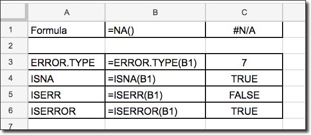
In fact, there is even a function to generate #N/A errors. It’s of limited use, but can be helpful for doing data validation in more complex formulas.
will output an #N/A error. (Google Docs Help on NA)
will return a number corresponding to the error type:
- 1 for #NULL!
- 2 for #DIV/0!
- 3 for #VALUE!
- 4 for #REF!
- 5 for #NAME?
- 6 for #NUM!
- 7 for #N/A
- 8 for all other errors
(Google Docs Help on ERROR.TYPE)
checks whether a value is the error #N/A, and will give the output TRUE for a #N/A error and FALSE otherwise. (Google Docs Help on ISNA)
checks whether a value is any error other than the #N/A error. (Google Docs Help on ISERR)
checks whether a value is an error, and will give the output TRUE for any error. (Google Docs Help on ISERROR)
These functions can be summarized in the following table:
13. Help! My formula is STILL not working
Take a deep breath, don’t panic! There’s an army of Google Sheets super users out there who would love to help you fix your issue, free of charge, in the active help forums.
Try posting your problem into the forum and someone will likely help you out.
To make it easier for people to help you, please share your Google Sheet in view-only mode(how to share your Google Sheet) and include the error message and what you were expecting the correct answer to be.
Great Resource
Where can I find information on the types of formula’s that will work in Google Sheets in the Data —›Filter—›Filter by condition… —›Custom formula is area?
I have much data that I need to filter by three columns in order to update it on a weekly basis. One field is a serialized number field (consisting of section#.meeting#.item#) of which I need to filter by meeting# only, another is a text field with a specified date in it with a format of “[mm/dd/yy]” and the third field is a data validated list.
This Google sheet has a header that references data from another sheet in the same workbook and the values that I need to filter by are returned in the header dropdown (VLookup) and shown on specific cell. Ideally, I would love to have the Custom Formula reference the values in these cells for the filter, but I am willing to enter them manually if I have to.
I need this Custom formula because I need to filter my data by the meeting# in the number field OR the specified date in the text field AND by the data validate list so that I can edit and append it.
I have another sheet that does a query of the data from this sheet with these parameters very well, but I cannot edit the data there. My specific challenge is how I can do an ArrayFormula in the Custom Filter field that mimics what I have done with the query() on my reporting sheet so that I can edit my data?
Good question! I don’t know of any specific resource for the formulas you can use inside of the filter. They need to start with an “=” sign, and you create a formula for the first row of your data, and let the filter apply that test to all the other rows, e.g. if your data was in A2:D100 say, with index numbers in column 1, and you wanted just odd numbers to remain, you could use a formula like “=isodd(A2)”.
Hope that helps! Feel free to share your sheet or a copy with dummy data if you want to delve further. Generally the formulas are not as comprehensive as what you can do in the general Google Sheet.
Somewhat related…
Is there a way to force a file to produce an error in Google Sheets….when the source is an Excel file? I’m wondering the case of someone taking my Excel file, uploading to Google Sheets – what I would love is for it to produce error messages all over the place to warn them that they can’t use in Google Sheets (needs to remain in Excel). Any advice? Thanks!
Hi, great article – thanks! I am having the issue with the closing brackets on my formula. Everytime I press enter, it adds quotation marks and a close bracket even though I have already put those in. Thus it doubles it up and produces an #ERROR! message. Any ideas?
Thank you if you can help!
Help ! i am trying to pull data from a cell in one tab on a spreadsheet to a cell on a second tab of same spreadsheet and when I enter the formula in the cell =’name of tab’!C1 (as cell number where data exists that I want to copy) and I get a pop up message saying cannot find ‘name of tab’ copy from : and it wants me to give a file on my computer that it is supposed to find this info. But it is right thhere on same xls sheet on a different tab name
Hi Jen – sounds like you’re using Excel? The info on this page applies to Google Sheets only. That being said, if you’re in the same spreadsheet you should have no trouble linking to a different tab within that spreadsheet. Just try clicking to the cell rather than typing in the cell reference.
Hi Ben – I am following both your courses ‘advanced formulas’ and ‘apps script’. Love it! From zero to pretty cool sheets in a week or two :-).
I am stuck on a reference issue. Maybe you could point me in the right direction:
sheet.getRange(2,5).setFormula(‘=ArrayFormula(
if(not(isblank($C$2:$C)),
$C$2:$C*$D$2:$D*calculatePrice(b2),” “))’);
This line of code is part of a script. It simply multiplies a value in the C-range with a value in the D-range with a price that is calculated with the function calculatePrice. The function takes a parameter (a label found in the B-Range – validated data) upon which it loops through an object to find a matching price. All of that works, but cell B2 should be B3 in the next line, B4 in the line after that etc. How do I get this to work in this formula? I have tried B2:B but that does not work. I have also used index() by omitting the row like so, index(B2:B, ,1) – it’s in the course :-). This works in a regular spreadsheet, but seems to fail in the context of my formula. Help is much appreciated, thanks JP
When I use SUM it seems as though only column D does not add all the numbers, it skips the first 20 lines. I do use as example =SUM(D3: D42)
all other columns add all the numbers correctly. Once I started double checking the addition I tried adding a column before the D which made the original C a D the new D column adds all the numbers. Very strange I realize we should always check our numbers but thought someone might have the same issue or might not realize and go by the SUM answer and be incorrect.
Amazing post. A question on this: i got some cells with #REF error. Some of them are “good” (= e.g. “importrange can’t expand”) some other are “bad” (= e.g. “internal error”).
As you know, you can get this kind of error just through mouseover. I do wander if there’s any way to get this content in another cell to use conditional formatting to spot that “bad” errors.
thanks
I am using this formula to calculate a students overall grade for the school year. Unfortunately the answers are wrong. The K6 field is a linked % grade for another sheet. Please help me to identify my error in this : =IF(ISERROR(I6*0.85+K6*0.15),”-“,ROUND(I6*0.85+K6*0.15,0))
Hello, I have tried everything, but I am still receiving this message.
– I am trying to get the sum of cell ‘B2 to B91’
– I have entered =sum(B2:B91) in cell B92
-“Error
The formula in cell B2:B92 is referencing a range in the active filter
Please assist
Hi there, I hope this forum is still active because I have a very particular issue that I am trying to solve. Basically- I have information on one sheet that I would like to put on my current sheet based on a key word. I used the functions LOOKUP and IMPORTRANGE for this task and was successful. Every value that I needed was pasted into the appropriate cell. This was for a sheet from last pay period. I copied the same sheet, deleted the information and filled it with this pay period’s info. When it came time to draw that same information from the sheet that I took it from before, I simply used the formula that I used last time. It doesn’t work and I cannot figure out why. It is the exact same formula and should draw information from the sheet I specified but doesn’t. It simply returns the N/A error and states that it hasn’t found said search keys. This formula works perfectly fine on an identical sheet. I even went as far as to change sharing rights and owners of certain sheets to make them as accessible as possible and still nothing. I also created a new sheet, put the information from the sheet that I pulled from before and used that HTML in the evaluation instead and it still returned the same error.
I have a formula that returns a value when a condition is met and returns null when not. From that column, I’m trying to build a query to create a count distribution but I want to exclude where the value is returned as null.
It is returning a lot of junk in query output column header when I use clause “where G is not null” where column G has the formula value. If I remove the clause, then I see the row with a null value and a count.
Any help to sort this out will be highly appreciated.
=if(FA3=FG3,“”,“Mismatch”)
What is wrong above ? I am still getting parse error.
If you simply do FA3=FG3 IT WILL RETURN TRUE OR FALSE THAT WILL SERVE THE PURPOSE
Then probably you can add if function like if(FH3= TRUE, ” ” ,”MISMATCH”)
Hi,
When i am putting formula with cell references like “C20*D20” value is coming as 1818.12 with C20 = 227.27 and D20 = 8.
Actually that’s not correct, since 227.27*8 = 1818.16
PARSE ERROR
Appears that in one Workbook – This works
=SUMPRODUCT(COUNTIF(B1,”*”&A5:A30&”*”)*(A5:A30″”))
But if I put it in another workbook that has a similar structure – it DOES NOT WORK – UNLESS
I change comma to semi-colon
Robert – sounds like it might be something to do with the spreadsheet locale affecting the syntax. See if this helps: https://www.benlcollins.com/spreadsheets/sheets-location/
This is very possible. Commas are used in US and semi colons in EUROPE. So, you might want to check the region settings of your workbook.
Here’s a free google-sheet formula parse and evaluate tool for untangling formulae:
https://docs.google.com/spreadsheets/d/1wwclmAMXGaFanVLlyvzv63fDx6JkwOcT6Dkisac-sXI/copy
It’s free. It’s tiny. It’s just a simple shared google-sheet file (with no macros, add-ons or fancy stuff). Click the link to make your own copy. Have a try, and if you like it, bookmark it for future use while fighting formulae in google-sheet.
I made it to make up for the lack in google sheet of the Evaluate Formula (F9) parser native to Excel. It analyses any formula pasted into yellow cell G1, splitting and colouring them by depth or by chosen characters, and referencing them against the available formulae to see where brackets or commas are likely to have been omitted or put in the wrong place. A handy tool for simple checks, and for making or parsing complex or nested formulas, and for finding ‘Parse Error’, and diagnosing #REF!, #NAME?, #N/A, #NUM!, #VALUE! error codes.
Enjoy!
I have a query that has no “errors”, however the output is omitting data from the source data. I believe it is because my source data has blank cells in it, which is correct as some of the columns are Descriptions and a null cell is correct, unfortunately even when some of the columns do have data in it, the query is showing up blanks for only some rows (not all). Has anyone else experienced this? Does Google query not like source data with nulls in them? I cant simply filter out nulls as i need the data in the rest of the row.
=networkdays(a1,b1)
This formula still error
Answer
#name
How do I fixed it
Thanks in advance
Is there a method in google app script to get the error message (what you see when mousing over the error cell)? I’m new to JS but want to write a script that finds #REF errors when an arrayformula won’t expand down because there is something in a cell below. I need part of the logic to read the error message to know it’s the right type of #REF error. Thanks so much.
Hi,
When I import a csv file in Gsheet, the data is correctly shown in columns, but it is impossible to sum the content of each column: the formula e.g. (=sum(e3:e30) is accepted but the sum is always 0.
Data pasted (even pasted as values) to other colums cannot be summed either: sum is always 0. Google Sheets sees imported values not as values?!
I’m trying to get an average for a specific cell range but exclude if the cell contains text (conditional format). I thought this would work, but doesn’t in sheets. Any suggestions? The text is specifically three lower case o’s.
=AVERAGEIF(B15:AF15, “ooo”)
Dear Ben,
You blogs and articles related to Google Spreadsheet really awesome.
I shall be very thankful to you if you could really help me on “Importrange Internal Error” which i am facing on large scale. all my sheets has stopped working due to this error if i found this error i usually cut and paste formula in cell and it starts working but in number of spreadsheet it is difficult for me to find and fix this error.
Request you to let me know the cause of error and give tips and solution to resolve this error.
Thanks in advance
Hello!
I’m trying to filter a query like what is below, but I keep turning up with the #Value error. When I remove the “Where K = ‘Absent’” part, it works. What am I doing wrong?
=FILTER(QUERY(‘Master Sheet’!A2:K, “Select D, E, F, G, J, K WHERE K = ‘Absent’ order by J desc”), WEEKNUM(‘Master Sheet’!A1:A)=WEEKNUM(NOW()))
Thank you
U16 = 2584034261
N17 = 2584034261
N18 = 2685921053
N19 = 2787807846
is there something wrong with this formula?
=IF(U16=N18;1;IF(U16(N17+((N18-N17)/2));((N17+((N18-N17)/2))-U16)/(N18-(N17+((N18-N17)/2)));IF(U16>N18 AND U16<N18+((N19-N18)/2);(U16-N18)/((N18+((N19-N18)/2))-N18);0)))
The following Info category functions may also help save the day here.
This last week I have been trying to troubleshoot some array formulas and was completely flumexed by not being able to confirm the reference that was being passed to one part of the function, i.e. the reference was constructed from indirect(), offset(), and switch().
Here, you can start by seeing if the refence your generating is even valid by using ISREF(), which returns TRUE when given a valid cell reference. Please note, that you’ll have to actually surround this part of your formula with this function, as using a reference to another cell would of course just confirm that first reference.
Okay, so now you know that you’re actually generating a reference, but how to confirm what that reference actually is?
Well the CELL() function has an option for using the word “address”, as it’s first argument, to return, in plain text, an absolute reference for the top left cell in reference a given reference. Then the range of that reference can be confirmed using the COLUMNS() and ROWS() functions together, and of course all three functions can be concatenated into a single string.
Thank you for all the effort and consideration that goes into these tutorials.
I am getting error in query formula for one column where I am getting error that row size is mismatch expectiing 184 actual 4. Please guide me how can I rectify it.
very very helpful!
Great tutorial! Thanks so much for this comprehensive article. Finding all fixes in one place is amazing.
Thanks a lot for the great article! Google Sheets is indispensable in my work. Often you have to do some kind of global analysis of the issue, and it is convenient to work in tables. Thank you!
Very useful hints.
I got a parse error in formulas because this cell has a reference to another sheet. (like =Sheet4!A1).
The problem arises when “Sheet4” is recreated during execution of apps script.
Manually clicking on the cell it is ok recalculated. but how to do it programatically by apps script?
Many thanks!