Array Formulas have a fearsome reputation in the spreadsheet world (if you’ve even heard of them that is).
Array Formulas allow you to output a range of cells, rather than a single value. They also let you use non-array functions with arrays (think ranges) of data.
In this post I’m going to run through the basics of using array formulas, and you’ll see they’re really not that scary.
Hip, Hip Array!
What are array formulas in Google Sheets?
First of all, what are they?
To the uninitiated, they’re mysterious. Elusive. Difficult to understand. Yes, yes, and yes, but they are incredibly useful in the right situations.
Per the official definition, array formulas enable the display of values returned into multiple rows and/or columns and the use of non-array functions with arrays.
In a nutshell: whereas a normal formula outputs a single value, array formulas output a range of cells!
The easiest way to understand this is through an example.
Imagine we have this dataset, showing the quantity and item cost for four products:
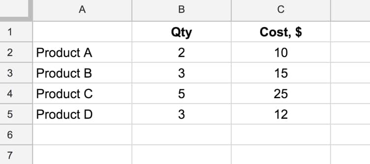
and we want to calculate the total cost of all four products.
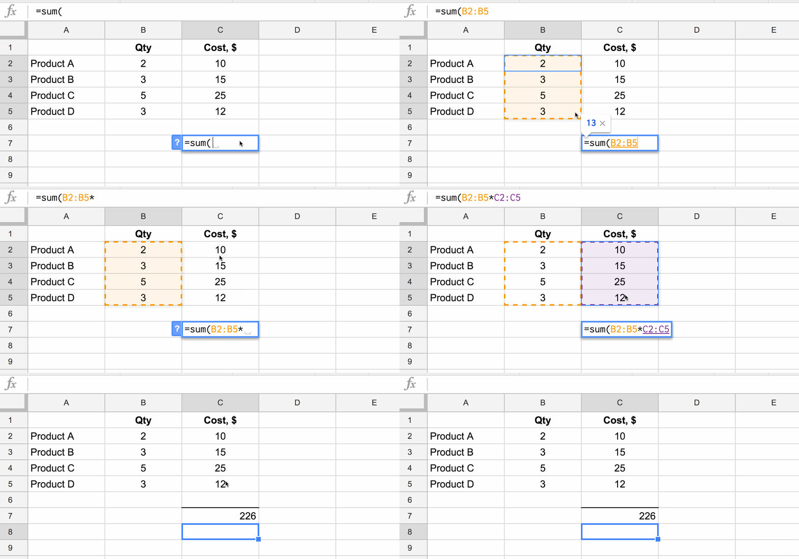
We could easily do this by adding a formula in column D that multiplies B and C, and then add a sum at the bottom of column D.
However, array formulas let us skip that step and get straight to the answer with a single formula.
 💡 Learn more
Learn more about working with Advanced Formulas in the Advanced Formulas in Google Sheets course
What’s the formula?
=ArrayFormula(SUM(B2:B5 * C2:C5))How does this formula work?
Ordinarily, when we use the multiplication (*) operator in a Sheet, we give it two numbers or two cells to multiply together.
However, in this case we’re giving it two ranges, or two arrays, of data:
= B2:B5 * C2:C5However, when we hit Enter this gives us a #VALUE! error as shown here:
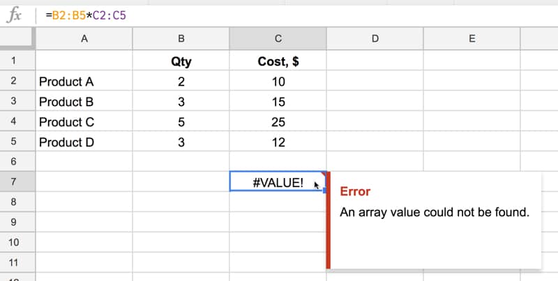
We need to tell Google Sheets we want this to be an Array Formula. We do this in two ways.
Either type in the word ArrayFormula and add an opening/closing brackets to wrap your formula, or, more easily, just hit Ctrl + Shift + Enter (Cmd + Shift + Enter on a Mac) and Google Sheets will add the ArrayFormula wrapper for us.
=ArrayFormula(B2:B5 * C2:C5)Now it works, and Google Sheets will output an array with each cell corresponding to a row in the original arrays, as shown in the following image:
Effectively what’s happening is that for each row, Google does the calculation and includes that result in our output array (here showing the equivalent formulas):
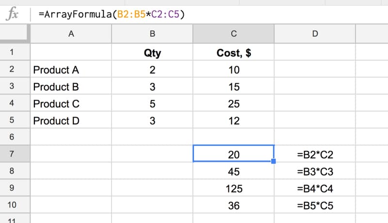
and another view, showing how the calculation is performed (just for the first and last row):
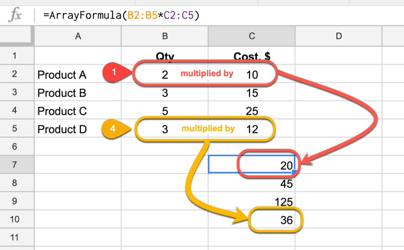
Note: array formulas only work if the size of the two arrays match, in this case each one has 4 numbers, so each row multiplication can happen.
Finally, we simply include the SUM function to add the four numbers:
=ArrayFormula(SUM(B2:B5 * C2:C5))as follows:

Quick Aside:
This calculation could also be done with the SUMPRODUCT formula, which takes array values as inputs, multiplies them and adds them together:
=SUMPRODUCT(B2:B5 , C2:C5)Another Array Formula Multiplication Example
In this example, we enter a single formula to multiply an array of row headings against an array of column headings.
This only works because the dimensions of the arrays are compatible, since the number of columns in the first matrix is equal to the number of rows in the second matrix:

Array Formula With IF Function
This is an example of a non-array function being used with arrays (ranges). It works because we designate the IF formula as an Array Formula.
Consider a standard IF statement which checks whether a value in column A is over $2,000 or not:
=IF(A2>2000,"Yes","No")This formula would then be copied into each row where we want to run the test.
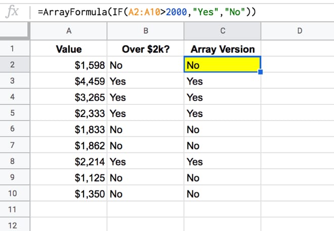
We can change this to a single Array Formula at the top of the column and run the IF statement across all the rows at once. For example, suppose we had values in rows 2 to 10 then we create a single Array Formula like this:
=ArrayFormula(IF(A2:A10>2000,"Yes","No"))This single formula, on row 2, will create an output array that fills rows 2 to 10 with “Yes”/”No” answers, as shown in the following image:
Can I see the example worksheet?
Click here to make your own copy



Hai, i trying to add Vlookup function from the response sheet collected from form, but the formula always goes down below 1 column whenever new data inserted from google form
can you post a picture of this?
Hello!… Is possible to use array formula in combination with text concatenation?
I could never get it to work with Arrayformula(Concatenate(x:x,y:y,z:z)) properly.
I replaced it with Arrayformula(X:X&Y:Y&Z:Z) and use this everyday.
If you need to repeat a Static Value
Arrayformula(X:X&$Y1&Z:Z) will work
Hey Ben,
Can you talk about arrayformulas and aggregation functions, like countifs, AND, sumifs?
In my experience, the array formula is inconsistent in it’s automatic expansion down a column. Is there a trick to making that happen? I often revert back away from arrayformulas and dragging the cell all the way down because my arrayformula’s do not expand.
My recent example.
Column A, check boxes, some checked, some not.
Column B, same as A
Column C, I want to check if EITHER A or B is checked. Using this formula: =ARRAYFORMULA(IF(OR(A1:A=TRUE,B1:B=TRUE),TRUE,FALSE)
When I enter this, it checks for Trues across entire columns, rather than calculating them by row, and doesn’t expand. What am I missing?
Found that this happens when using BOOL checks within the IF. My workaround is to rework the logic as nested IFs instead – can get a bit messy but it works.
IF A then TRUE; ELSE-IF B then TRUE; ELSE FALSE
Which would look like:
=ARRAYFORMULA(IF(A2:A=TRUE,TRUE,IF(B2:B=TRUE,TRUE,FALSE)))
If you would like it to only be applied to the rows where A is not empty then you could add an initial check for this:
=ARRAYFORMULA(IF(A2:A””,IF(A2:A=TRUE,TRUE,IF(B2:B=TRUE,TRUE,FALSE)),))
If you wanted the initial check to be A AND B instead:
=ARRAYFORMULA(IF(A2:A””,IF(A2:A=TRUE,IF(B2:B=TRUE,TRUE,FALSE),FALSE),))
Hi there – I have a set of nested IF() that includes AND() that works fine but when adding ARRAYFORMULA() it does not automatically expand. I still have to drag the formula down to fill the cells. I can’t figure out what I am doing wrong – can anyone give me any hints of things to look for?? Thanks!
Can you post a sample of the formula?
and formula for array
Hey, what is the best practice for Google Sheets with large volumes of data (200,000 + rows). Is an ArrayFormula or a pasted down formula going to be more efficient and better database management?
For example, would:
‘=ArrayFormula(IF(ISBLANK(A2:A),,A2:A&”_”&H2:H&”_”&K2:K&”_”&D2:D))’
be a better solution or
‘=A2&”_”&H2&”_”&K2&”_”&D2’ and then pasted down?
Hey! Thank you so much for the content. I really appreciate the detailed explanations!
I’m trying to use the ArrayFormula to flatten a table, but I needed to leave the range conditioned to the last row where there’s data, so when I have a new entry, the flattened table is automatically generated.
I’ve tried several ways (with address, indirect, and others), but nothing worked so far. Do you have any tips where I can look for?
TIA!
Hi Camila,
Have a look at this post on how to flatten a table, it might help: https://www.benlcollins.com/spreadsheets/unpivot-in-google-sheets/
Cheers,
Ben
I have used arrey formula with multiple condition, however its getting delete with new response.
=Arrayformula(IF(F2=”First”,1,IF(F2=”Second”,2,IF(F2=”Night”,3,IF(F2=”General”,4,”No Shift”)))))
Request your support
F2:F
I have used arrey formula in google form response sheet with multiple condition, however its getting delete with new response.
=Arrayformula(IF(F2=”First”,1,IF(F2=”Second”,2,IF(F2=”Night”,3,IF(F2=”General”,4,”No Shift”)))))
Request your support..!
Hi,
Thank you for sharing the article. I tried doing what you shared about not getting the formula skipped to next row whenever we have a new response added. Tried using ISBLANK but the error pertains i.e. whenever a new response is added, the formula is just skipped to the next row and does not perform function to recently added one.
Need your help here!
Thanks so much .
I’d like to capture the sum of labor hours per account on a different sheet. Ideally it would adjust automatically as data is entered. I have not found a way to do this with CountIf and I think Array Formulas are where I need to look, but I am not sure.
Example:
Date | Acct Name | Labor Hours
3/4 Steve 3
3/5 Mark 2
3/6 Mark 1
3/7 Steve 4
In the example, I would like the formula to capture the total the hours per account on another sheet like so:
Acct Name | Total Labor Hours
Steve 7
Mark 3
Thank you for any assistance.
What is the advantage with an ArrayFormula in your last example?
And could an ArrayFormula be used when you apply conditional formatting? E.g., say that you want to highlight cells in column B if they are different from the cell in column A on the same row. In other words, B1 should be compared with, only, A1, B2 only with A2, B3 with A3 etc.